90. 1993 Prospects for Bounded Rationality in Macroeconomics#
90.1. Overview#
This is the closing lecture of the series, and it is different in kind from the others.
It carries no new model.
Instead it gathers the judgments that Sargent [1993] recorded in 1993 — the opinions, reservations, and hopes with which he ended Bounded Rationality in Macroeconomics — and loops them back to the quest that opened the book, and that opened A Peculiar Definition of Bounded Rationality, the first lecture here.
That quest had a destination: a theory of transition dynamics, the out-of-equilibrium adjustment that the Eastern European reformers of 1989 had to manage with no map.
The route was to expel the rational agents from our models and replace them with “artificially intelligent” agents who behave like econometricians, who gather data, form theories, estimate, and adapt.
We can now ask how far that route carried us, by 1993, toward the destination.
Sargent’s own answer is a ledger, with entries on both sides.
On the credit side: adaptive dynamics as a device for selecting among equilibria, and as a tool — evolutionary programming — for computing them.
On the debit side: the original prize, a theory of transition dynamics, is largely unclaimed; and a striking asymmetry has emerged.
The program set out to make the agents in our models behave more like econometricians.
The econometricians, Sargent observes, have not returned the compliment.
This lecture explains that asymmetry, gives it a concrete numerical face, and reads the ledger against the opening quest.
The lecture then closes with a postscript on what became of the program after 1993.
Let’s start with some imports.
import numpy as np
import matplotlib.pyplot as plt
90.2. The quest, restated#
It is worth restating the argument of the first lecture, because everything below is measured against it.
Rational expectations imposes two requirements: individual rationality, and mutual consistency of perceptions.
The second is the demanding one, and — this is the crux — when a rational expectations model is taken to data, it imputes far more knowledge to the agents inside it than to the econometrician studying them.
The agents evaluate their Euler equations using the equilibrium probability distributions, the very distributions the econometrician is still struggling to estimate.
The bounded rationality program proposes to close that gap by demoting the agents to the econometrician’s own level: they too must learn the distributions, from data, as they go.
The hope was that this would deliver something rational expectations cannot: a description of the system while it is still adjusting, before beliefs and outcomes have settled into mutual consistency.
That is what a theory of transition dynamics would be.
We now take stock, following Sargent [1993]’s own accounting: first the debits, then the central asymmetry, then the credits.
90.3. The debit side: how much we must hard-wire#
The first reservation is about arbitrariness.
Bounded rationality is most easily defined by what it is not — rational expectations — and that very malleability is a liability.
Once we stop insisting that agents know the equilibrium, we must decide, case by case, exactly what they do know and how they learn it.
Do they know their own utility and profit functions, or must they learn those too?
Do they know calculus and dynamic programming, or only trial and error?
Do they learn from their own experience alone, or from others’?
To what class of approximating functions do we confine what they learn about?
Every model in this series answered these questions by hard-wiring, by prompting the agents heavily, with an eye on the outcome we hoped they would reach.
Bray’s agents, in A Peculiar Definition of Bounded Rationality’s adaptive-expectations model and in the least squares learning literature, know the correct supply curve and need only estimate one conditional expectation to plug into it.
The Marcet–Sargent agents know dynamic programming, know their return function, and know the parametric form of the law of motion — they lack only its coefficients, which they update by vector autoregression.
Even the classifier agents of Money as a Medium of Exchange among Artificially Intelligent Agents, which are prompted far less — they are never told their utility functions, and recognize utility only when they experience it — are still told when to choose and what information to condition on, and the entire apparatus of their accounting system and genetic operators is designed by hand, with the Kiyotaki–Wright equilibrium in view.
The second reservation is about simplicity.
The learning tasks we set our agents are trivial next to those in a first econometrics course, let alone those that real firms and households are implicitly solving.
We ask an agent to learn a single time-invariant decision rule, or a fixed collection of conditional expectations.
We do not ask it to learn the parameters of a simultaneous-equations system, or to infer a mapping from policy regimes to distributions, the tasks that make econometrics hard.
Put together, these reservations bear directly on the original prize.
The environments into which we have cast our adaptive agents are far more stable and hospitable than the transitions we actually care about.
Convergence-rate results are scarce, and tractability forces us to restrict the distribution of agents’ beliefs severely.
So the literature on adaptive processes, Sargent judged in 1993, falls well short of a secure foundation for a theory of real-time transition dynamics, the very thing the quest set out to find.
He declines to end on that failure, though, and the baseball metaphor he reaches for is deliberately modest:
It would not be wise or fair to end this essay by dwelling on the failure of adaptive methods so far to have ‘hit a home run’ by giving us a good theory of transition dynamics. The problem of transition dynamics is difficult and long-standing. So maybe it should count as a single, or at least a sacrifice fly, that these methods have sharpened our appreciation of the problem.
90.4. Why the econometricians have not returned the compliment#
Here is the asymmetry that gives this lecture its theme.
The bounded rationality program is, at bottom, a movement to make the agents in our models behave more like the econometricians who build and estimate those models.
Imitation is the sincerest form of flattery.
We might therefore have expected macroeconometricians to rush to fit these models to data.
There was no rush.
Chung [1990]’s estimation of the Sims policy-maker model — the application in Adaptive Agents in an Overlapping Generations Monetary Economy — was, Sargent noted, close to the only econometrically serious macroeconomic implementation of bounded rationality he knew of.
Why the reluctance?
The reasons are worth spelling out, because they are not about taste.
The governing dictum among applied econometricians is Lucas’s: beware of theorists bearing free parameters.
Replacing a rational agent with a boundedly rational one adds parameters: parameters describing beliefs and how beliefs move.
Take the simplest case, Bray’s model.
Relative to its rational expectations version, the adaptive version adds at least the initial belief and a parameter setting the gain sequence, and one might want more parameters to describe the gain’s shape.
That would already give Lucas’s warning something to bite on.
But there is a deeper problem, and it is the reason the added parameters are not just unwelcome but genuinely hard to estimate.
Because the adaptive system converges to the rational expectations equilibrium, the extra parameters influence only the transient.
The asymptotic distribution of the data contains no information about them.
Let us see this directly.
90.4.1. The nuisance parameter, made concrete#
Bray’s cobweb economy [Bray, 1982] sets the market price by
where \(\beta_t\) is the price agents expect, formed by averaging past prices,
and \(u_t\) is an IID shock.
The constant \(t_0\) is the weight the agents attach to the belief they start with, measured in observations: with \(t_0 = 50\) they treat \(\beta_0\) as though it summarized fifty prior prices, so that after \(t\) periods \(\beta_0\) still carries weight \(t_0/(t + t_0)\).
Some such weight is needed for the exercise to have any content.
With \(t_0 = 0\) the first gain is \(\gamma_1 = 1\), so \(\beta_1 = p_0\) exactly and the initial belief is erased after a single period — there would be no transient left for the econometrician to try to estimate.
When \(b < 1\) the belief converges to the rational expectations value \(\beta^\star = a/(1-b)\), whatever value it started from.
a, b, sigma_u = 5.0, 0.7, 1.0
t0 = 50                                       # weight on the initial belief
β_star = a / (1 - b)                       # rational expectations belief

def simulate(β0, u):
    "Bray's cobweb under least squares learning, given a shock path u."
    T = len(u)
    β = np.empty(T)
    p = np.empty(T)
    β[0] = β0
    for t in range(T):
        p[t] = a + b * β[t] + u[t]
        if t + 1 < T:
            β[t + 1] = β[t] + (1 / (t + 1 + t0)) * (p[t] - β[t])
    return p, β

print(f"rational expectations belief β* = {β_star:.3f}")
rational expectations belief β* = 16.667
The initial belief \(\beta_0\) is the extra “bounded rationality” parameter.
Watch three economies with very different initial beliefs forget where they started.
rng = np.random.default_rng(0)
u = rng.standard_normal(400)

fig, ax = plt.subplots(figsize=(7.5, 4))
for β0, colour in [(2.0, 'C0'), (16.667, 'C1'), (40.0, 'C2')]:
    _, β = simulate(β0, u)
    ax.plot(β, color=colour, lw=1.3, label=fr"$\beta_0 = {β0}$")
ax.axhline(β_star, color='k', ls='--', lw=0.8, label=r"$\beta^\star$")
ax.set_xlabel("$t$")
ax.set_ylabel(r"belief $\beta_t$")
ax.legend(frameon=False)
plt.show()
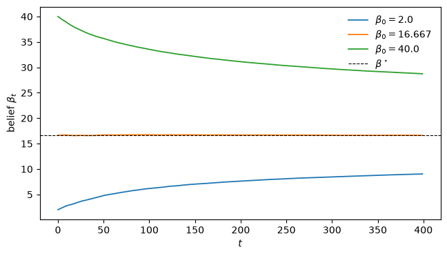
Fig. 90.1 The belief forgets its starting point#
All three converge to \(\beta^\star\).
Now put on the econometrician’s hat.
Given a sample of prices and the structural parameters \((a, b)\), the model implies a shock \(\hat u_t = p_t - a - b\,\beta_t(\beta_0)\) for any candidate initial belief \(\beta_0\), because the belief path is pinned down by \(\beta_0\) and the observed prices.
The sum of squared implied shocks measures how well a given \(\beta_0\) fits the data.
def belief_path(β0, p):
    "Belief sequence implied by an initial belief and an observed price path."
    T = len(p)
    β = np.empty(T)
    β[0] = β0
    for t in range(1, T):
        β[t] = β[t - 1] + (1 / (t + t0)) * (p[t - 1] - β[t - 1])
    return β

def ssr(β0, p):
    "Sum of squared implied shocks, as a function of the belief parameter β0."
    β = belief_path(β0, p)
    return np.sum((p - a - b * β) ** 2)
Whether the data can pin \(\beta_0\) down is a question of how fast information about it accumulates as the sample grows.
The natural way to read that off is the excess sum of squares — how much worse a wrong \(\beta_0\) fits than the best one.
For an ordinary, well-identified parameter every new observation adds to the penalty for being wrong, so the excess grows in proportion to \(T\) and the confidence interval shrinks like \(1/\sqrt{T}\).
Watch what happens here.
grid = np.linspace(2, 40, 80)

def excess_curve(T, seed=1):
    "SSR(β₀) − min SSR across the β₀ grid, for a sample of length T."
    u = np.random.default_rng(seed).standard_normal(T)
    p, _ = simulate(β_star, u)
    curve = np.array([ssr(b0, p) for b0 in grid])
    return curve - curve.min()

fig, ax = plt.subplots(figsize=(7.5, 4))
for T, colour in zip((50, 500, 5000), ('C0', 'C1', 'C2')):
    ax.plot(grid, excess_curve(T), color=colour, lw=1.5, label=f"$T = {T}$")
ax.axvline(β_star, color='k', ls='--', lw=0.8)
ax.set_xlabel(r"belief parameter $\beta_0$")
ax.set_ylabel("excess sum of squares")
ax.legend(frameon=False)
plt.show()
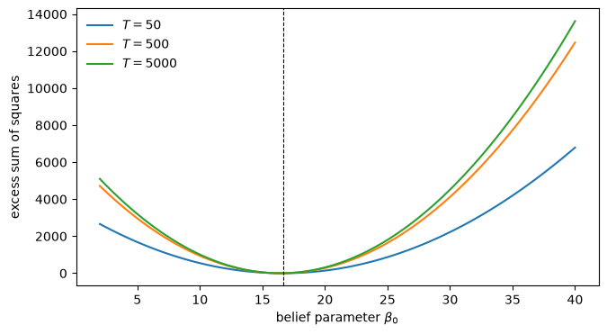
Fig. 90.2 Information about the belief parameter stops accumulating#
The curves stack on top of one another instead of getting steeper.
To see that this is not an artifact of the range plotted, compare the penalty for a wrong \(\beta_0\) with the penalty for a wrong slope \(b\), an ordinary structural parameter of the same model, estimated from the same data.
rows = []
for T in (50, 500, 5_000, 50_000):
    u = np.random.default_rng(1).standard_normal(T)
    p, _ = simulate(β_star, u)
    β = belief_path(β_star, p)                  # belief path at the true β0
    wrong_β0 = ssr(2.0, p) - ssr(β_star, p)
    wrong_slope = (np.sum((p - a - 0.75 * β) ** 2)
                   - np.sum((p - a - b * β) ** 2))
    rows.append([T, wrong_β0, wrong_slope])

for T, e_b0, e_b in rows:
    print(f"T = {T:6d}:  penalty for β₀ = 2 : {e_b0:10.1f}     "
          f"penalty for b = 0.75 : {e_b:12.1f}")
T =     50:  penalty for β₀ = 2 :     2662.3     penalty for b = 0.75 :         37.8
T =    500:  penalty for β₀ = 2 :     4714.1     penalty for b = 0.75 :        373.4
T =   5000:  penalty for β₀ = 2 :     5097.1     penalty for b = 0.75 :       3558.9
T =  50000:  penalty for β₀ = 2 :     5127.5     penalty for b = 0.75 :      35194.0
The two columns behave completely differently.
The penalty for getting the slope wrong grows in proportion to the sample: a hundredfold more data makes a hundredfold stronger case against the wrong value, which is what identification looks like.
The penalty for getting the initial belief wrong stops growing.
Past a few thousand observations it is pinned at a constant, and every further observation is uninformative about \(\beta_0\).
The confidence interval for \(\beta_0\) never shrinks; the parameter is not consistently estimable at all.
This is the technical heart of the matter.
The parameters that bounded rationality adds live entirely in the transient.
A transient contributes a fixed, finite amount of information no matter how long we watch the economy afterwards, so those parameters become a nuisance to estimate — they enter the likelihood, and the data have only ever a bounded amount to say about them.
And there is a final, decisive reason for the econometricians’ cool response.
Many applied macroeconometricians are in the market for methods that reduce the number of parameters needed to explain the data.
A reduction is precisely what bounded rationality does not offer.
It offers more parameters, most of them weakly identified.
So the flattery ran one way.
The theorists remade their agents in the econometrician’s image; the econometricians, offered models full of extra, poorly-identified parameters, and warned by Lucas against exactly that, declined the gift.
90.5. The credit side: selection, computation, and a returned gift#
The ledger is not one-sided.
Set against those debits, Sargent lists three genuine successes, and the last of them quietly undoes some of the asymmetry just described.
Equilibrium selection.
Where a rational expectations model has many equilibria, a system of adaptive agents often converges to a particular one, turning learning into a device for selecting among them.
We saw it repeatedly: the low-inflation equilibrium chosen in Adaptive Agents in an Overlapping Generations Monetary Economy, the history-dependent exchange rate of Exchange Rate Indeterminacy, Learning, and Experiments, the fundamental monetary equilibrium of Money as a Medium of Exchange among Artificially Intelligent Agents.
Sargent is candid that his affection for this use sits in some tension with his doubts about the dynamics that perform the selection:
I know that it is inconsistent to doubt the real-time dynamics but keep the equilibria selected by them. I confess that my affection for the selection performed in the monetary models described in Chapter 6 is partly driven by my prior conviction that the selected equilibria seem sensible to me.
Evolutionary programming.
If a population of adaptive agents reliably converges to an equilibrium, we can run the population as a method of computing the equilibrium, especially in models too complicated to solve by hand.
That is exactly what Money as a Medium of Exchange among Artificially Intelligent Agents did with the five-good Kiyotaki–Wright economy, for which no analytical characterization was in hand.
Sargent expected this use to be applied often.
New tools for the econometrician.
Here the asymmetry bends back on itself.
The literatures on parallel and genetic algorithms have handed econometricians new computational gadgets — genetic algorithms and stochastic Gauss–Newton procedures among them — for solving their own estimation and optimization problems.
McGrattan, for instance, used genetic algorithms to search for the neighborhood of a maximum before switching to a Newton method, a use noted back in Genetic Algorithms and Classifier Systems.
So the econometricians took up the adaptive algorithms after all, not as models of the agents they study, but as tools in their own hands.
The compliment was returned, but through a side door: the algorithms crossed over, the models did not.
90.6. Reading the ledger against the quest#
Line the two columns up against the destination we set out for.
The debit column holds the prize itself.
A theory of real-time transition dynamics — the map the Eastern European reformers lacked — remained, in 1993, largely unclaimed, blocked by arbitrariness, prompting, over-simple learning tasks, and a shortage of empirical traction.
The credit column holds what the journey delivered along the way: a principled way to select among multiple equilibria, a practical way to compute equilibria that resist analysis, and a transfer of computational technique into econometrics itself.
The organizing image of the whole book is the gap between the econometrician and the agents inside the model.
Rational expectations closes that gap by lifting the agents up to a knowledge the econometrician lacks.
Bounded rationality proposed to close it from the other side, by bringing the agents down to the econometrician’s level and making them learn.
By 1993 the program had not, on Sargent’s own accounting, delivered the transition dynamics that motivated it, and the econometricians it sought to imitate had kept the models at arm’s length — for the sound reason that those models add parameters the data cannot identify, when what the econometrician wants is fewer.
But it had sharpened the questions, selected equilibria, computed them, and lent its tools to the very econometricians who declined its models.
That was the state of the prospects for bounded rationality in macroeconomics, as they stood in 1993.
90.7. Postscript: what became of the program#
Three decades is long enough to see which of the 1993 worries were permanent and which were about a field that had not yet found its footing.
90.7.1. The arbitrariness was disciplined#
The first reservation was that once we stop insisting agents know the equilibrium, nothing tells us what to put in its place.
The discipline that emerged is expectational stability.
Evans and Honkapohja [Evans and Honkapohja, 2001] showed that whether a rational expectations equilibrium is learnable is governed by a condition on the map from perceived to actual laws of motion — the very \(T\) map of A Peculiar Definition of Bounded Rationality — and that the condition is largely independent of the details of the learning algorithm.
That is exactly what was missing in 1993.
Selection is no longer an artifact of whichever recursion the modeller happened to write down; a large class of reasonable learning rules select the same equilibria, and one can check which those are without simulating anything.
The stability reversal of Adaptive Agents in an Overlapping Generations Monetary Economy is a case in point.
It looked in 1993 like a fact about least squares, propped up by Bruno and Fischer [1990] having found the same thing with a different estimator.
E-stability explains why the two agreed.
90.7.2. The transition dynamics arrived, in a narrower form than hoped#
The prize was a theory of out-of-equilibrium adjustment.
What the program delivered instead was a theory of departures from equilibrium: escape dynamics.
The sawtooth we simulated at the end of Adaptive Agents in an Overlapping Generations Monetary Economy was, in 1993, a numerical curiosity.
Cho et al. [2002] characterized it analytically with large-deviations theory, computing the most likely escape path and the rate at which escapes occur, and Williams [2019] extended the characterization considerably.
The QuantEcon lectures Escaping Nash Inflation and Priors, Escapes, and Learning Cycles work through both.
This is less than the original quest asked for.
It describes recurrent excursions away from a self-confirming equilibrium, not the arrival of a market economy in a country that never had one.
But it is a genuine theory of a system that does not settle down, derived rather than simulated, and in 1993 there was none.
90.7.3. The econometricians did return the compliment#
Here the 1993 assessment was simply overtaken.
The obstacle, we saw above, was that the added parameters live in a vanishing transient.
But that argument applies only to a learning scheme with a \(1/t\) gain, which converges and then stops moving.
Constant-gain learning has no such transient. Beliefs never settle; they keep moving forever, and their movement is part of the stationary distribution of the data.
So the gain is identified the way an ordinary structural parameter is — from the whole sample, at the usual rate — and not, like \(\beta_0\), from a bounded initial episode.
Let us check that on the model we have been using.
def simulate_constant_gain(β0, gain, u):
    "Bray's cobweb when agents discount old prices at a fixed rate."
    T = len(u)
    β, p = np.empty(T), np.empty(T)
    β[0] = β0
    for t in range(T):
        p[t] = a + b * β[t] + u[t]
        if t + 1 < T:
            β[t + 1] = β[t] + gain * (p[t] - β[t])
    return p, β

def ssr_gain(g_hat, p, β0):
    "Fit criterion for a candidate gain, given observed prices."
    T = len(p)
    β = np.empty(T)
    β[0] = β0
    for t in range(1, T):
        β[t] = β[t - 1] + g_hat * (p[t - 1] - β[t - 1])
    return np.sum((p - a - b * β) ** 2)

gain_true = 0.05
for T in (500, 5_000, 50_000):
    penalties = []
    for seed in range(20):                    # average out sampling noise
        u = np.random.default_rng(seed).standard_normal(T)
        p, _ = simulate_constant_gain(β_star, gain_true, u)
        penalties.append(ssr_gain(0.08, p, β_star) - ssr_gain(gain_true, p, β_star))
    print(f"T = {T:6d}:  mean penalty for using gain 0.08 instead of 0.05 : "
          f"{np.mean(penalties):9.1f}")
T =    500:  mean penalty for using gain 0.08 instead of 0.05 :       1.1
T =   5000:  mean penalty for using gain 0.08 instead of 0.05 :       9.8
T =  50000:  mean penalty for using gain 0.08 instead of 0.05 :     123.6
The penalty grows in proportion to the sample, exactly as it did for the slope \(b\) and exactly as it did not for the initial belief.
That is why the econometric work that eventually materialized uses constant gain.
Sargent et al. [2006] estimated a constant-gain learning model of the Federal Reserve on post-war U.S. data — imputing to the government inside the model a genuine recursive estimation procedure, and asking the data which gain it used.
Sargent and Williams [2005] studied how the government’s prior about drifting coefficients shapes what it converges to, and Priors, Escapes, and Learning Cycles develops that.
Drifts and Volatilities fits a drifting-coefficient VAR to the same episode and asks whether it was bad policy or bad luck.
So the flattery did run both ways in the end.
It took a change in the learning technology — from a scheme that converges to one that never does — to make the models estimable, and that change was made for reasons of economics rather than econometrics.
90.7.4. A second retreat, made differently#
The program in this book keeps individual rationality and gives up mutual consistency: agents optimize, but against beliefs they are still estimating.
A parallel literature retreats along the other axis.
In the robustness work of Hansen and Sargent [Hansen and Sargent, 2008], agents do not estimate their model at all.
They admit that they cannot know it, and optimize against the worst case among the models they cannot rule out.
The two are complements rather than rivals, and both are answers to the question that opens A Peculiar Definition of Bounded Rationality: what do we do about the knowledge that rational expectations imputes?
One answer is that agents should learn what the econometrician is learning.
The other is that they should behave well without ever learning it.
90.7.5. The algorithms kept crossing over#
The 1993 ledger noted that econometricians had adopted the adaptive algorithms as computational tools even while declining the models.
That traffic increased, and reversed direction again.
Holland’s bucket brigade of Genetic Algorithms and Classifier Systems — pay part of your reward backward to whatever set you up — is temporal-difference learning, which became the organizing idea of modern reinforcement learning [Sutton and Barto, 2018].
The classifier systems of Money as a Medium of Exchange among Artificially Intelligent Agents are recognizable, in retrospect, as reinforcement learners with a hand-built function approximator; and the perceptrons of Genetic Algorithms and Classifier Systems became the deep networks of Introduction to Artificial Neural Networks, which now serve as the function approximators.
Sargent’s artificially intelligent agents were not, it turned out, a metaphor borrowed from a neighboring field.
They were an early instance of what that field went on to build.
90.7.6. Reading the ledger again#
The 1993 debits have not all been paid.
The choices remain many, the learning tasks we set our agents remain simple next to the ones real firms solve, and no one has produced the theory of transition dynamics that the Eastern European reforms called for.
But the entries have moved.
Selection acquired a theory instead of a set of examples; non-convergence acquired an analytical characterization instead of a simulation; and the econometricians, offered a version of the models whose extra parameters the data could actually speak to, took them up.
The gap between the econometrician and the agents inside the model is still there.
It is narrower, and we now know a good deal about its width.