86. Learning, Approximation, and Equilibrium Computation#
86.1. Overview#
In Adaptive Agents in an Overlapping Generations Monetary Economy a system of adaptive agents found a rational expectations equilibrium it was never told about.
The agents there learned a separate saving rate for each level of the government deficit — a non-parametric rule, one number per state.
That works when there are two states.
It runs into two walls otherwise, both noted in Sargent [1993]:
a state that occurs rarely is learned about slowly, because its observations arrive slowly;
when the number of states is large — and especially when the state is continuous — one parameter per state is hopeless.
The econometrician’s response is to impose a parametric form on the decision rule, \(s = f(G, \theta)\), with \(\theta\) of low dimension, and use every observation to estimate \(\theta\).
This lecture works through what that buys and what it costs.
The costs and benefits are two sides of one idea.
A parametric family can be learned quickly because every observation informs every state.
But a learning scheme confined to a family of functions can converge to a rational expectations equilibrium only if some member of the family supports one.
Otherwise the best it can reach is an approximate equilibrium.
Working this out surfaces a theme that runs through the whole bounded-rationality program:
Learning algorithms and equilibrium computation algorithms look like each other.
We will make that concrete.
Marcet’s method of parameterized expectations — a standard tool for computing rational expectations equilibria — turns out, when written recursively, to be exactly a model of adaptive agents learning.
An equilibrium computation is a centralized learning algorithm run by the modeller; a learning economy is a decentralized equilibrium computation run by the agents.
The plan:
Put a continuous deficit into the overlapping generations model of the previous lecture, turning the equilibrium condition into a functional equation in the saving rule \(f(G)\).
Compute a benchmark solution, so we have ground truth to measure against.
Solve it by parameterized expectations with families of increasing richness, and watch approximate equilibria give way to the exact one.
Show that the recursive, real-time version of the same algorithm is a learning economy.
Learn the saving rule non-parametrically with a kernel estimator, and weigh the trade-off against the parametric route.
Let’s start with some imports.
import numpy as np
import pandas as pd
import quantecon as qe
import matplotlib.pyplot as plt
from scipy.optimize import brentq
86.2. A continuous-state functional equation#
We keep the overlapping generations monetary economy of Adaptive Agents in an Overlapping Generations Monetary Economy — two-period lived agents, log utility, endowments \(w_1\) when young and \(w_2\) when old, currency the only store of value, and a government financing a deficit by printing money.
The one change: the deficit \(G_t\) now follows a continuous Markov process, with transition kernel \(F(G', G) = \operatorname{Prob}\{G_{t+1} \leq G' \mid G_t = G\}\).
We look for a stationary equilibrium in which saving is a function of the current deficit, \(s_t = f(G_t)\).
The household’s first-order condition, evaluated at \(s_t = f(G_t)\), is
and the government budget constraint with market clearing gives the return on currency in terms of the saving rule, exactly as before (with \(N = 1\)),
Substituting \(R_t\), and using \(f(G_t) R_t = f(G_{t+1}) - G_{t+1}\) for old-age consumption, turns the first-order condition into a functional equation in \(f\):
Under log utility, \(u'(c) = 1/c\), and because \(f(G_t)\) is known at \(t\) it pulls out of the expectation.
Writing
equation (86.1) becomes
So the whole problem reduces to finding the conditional expectation \(\psi(G)\): once we have it, the saving rule follows in closed form.
That observation is the hinge of the entire lecture.
Every method below — parametric or not — is a way of estimating the one object \(\psi(G)\).
w1, w2 = 20.0, 10.0

def s_from_psi(ψ):
    "Recover the saving rule from the conditional expectation ψ."
    return w1 * ψ / (1 + ψ)
86.2.1. The deficit process#
We take \(\log G_t\) to follow an AR(1), \(\log G_{t+1} = (1-\rho)\log \bar G + \rho \log G_t + \sigma \varepsilon_{t+1}\), and discretize it with the method of Tauchen [1986] to get a fine grid for the benchmark.
The parameters keep the deficit modest enough that a monetary equilibrium exists at every state.
ρ, σ, G_bar = 0.7, 0.30, 0.6

mc = qe.tauchen(21, ρ, σ, mu=np.log(G_bar) * (1 - ρ), n_std=2.5)
G, P = np.exp(mc.state_values), mc.P
ergodic = mc.stationary_distributions[0]      # where the deficit spends its time

print(f"deficit grid: {len(G)} points from {G.min():.3f} to {G.max():.3f}")
print(f"mean deficit under the ergodic distribution: {ergodic @ G:.3f}")
deficit grid: 21 points from 0.210 to 1.715
mean deficit under the ergodic distribution: 0.654
86.3. A benchmark solution#
To measure any learning scheme, we first need the true \(f(G)\).
On the discrete grid, (86.1) is a system of equations that we solve by iterating the perceived-to-actual map, precisely the \(T\) map of A Peculiar Definition of Bounded Rationality.
Guess a saving rule; use it on the right-hand side to compute the actual saving each state would call forth; repeat until the two agree.
Because \(\psi\) is monotone we can invert the first-order condition state by state with a bracketing root-finder, which makes the iteration robust.
def solve_benchmark(G, P, damp=0.5, tol=1e-12, max_iter=5000):
    "Fixed point of the perceived-to-actual saving map on the deficit grid."
    n = len(G)
    s = np.full(n, (w1 - w2) / 2)
    for it in range(max_iter):
        s_new = np.empty(n)
        for i in range(n):
            # E_t[ u'(c2) (s' - G') ] under the perceived rule s
            expect = sum((s[j] - G[j]) / (w2 + (s[j] - G[j])) * P[i, j] for j in range(n))
            # solve  1/(w1 - s_i) = expect / s_i  for s_i in (G_i, w1)
            foc = lambda si: 1/(w1 - si) - expect/si
            s_new[i] = brentq(foc, G[i] + 1e-9, w1 - 1e-9)
        if np.max(np.abs(s_new - s)) < tol:
            return s, it
        s = damp * s_new + (1 - damp) * s
    return s, it


s_benchmark, iters = solve_benchmark(G, P)
print(f"converged in {iters} iterations")


def foc_residual(s_rule):
    "Max |first-order-condition error| of a saving rule under the true kernel P."
    n = len(G)
    err = []
    for i in range(n):
        rhs = sum((s_rule[j] - G[j]) / (w2 + (s_rule[j] - G[j])) / s_rule[i] * P[i, j]
                  for j in range(n))
        err.append(1/(w1 - s_rule[i]) - rhs)
    return np.max(np.abs(err))


print(f"benchmark FOC residual: {foc_residual(s_benchmark):.2e}")
print(f"saving rule f(G) runs from {s_benchmark.max():.3f} (low deficit) "
      f"to {s_benchmark.min():.3f} (high deficit)")
converged in 224 iterations
benchmark FOC residual: 2.16e-14
saving rule f(G) runs from 4.470 (low deficit) to 2.831 (high deficit)
fig, ax = plt.subplots(figsize=(6.5, 4))
ax.plot(G, s_benchmark, 'k-', lw=2)
ax.set_xlabel("deficit $G$")
ax.set_ylabel("saving $f(G)$")
plt.show()
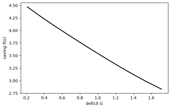
Fig. 86.1 Benchmark equilibrium saving rule#
Saving falls as the deficit rises: a larger deficit means faster money creation, a poorer return on currency, and less saving.
The rule is gently curved, which will matter in a moment.
This \(f(G)\) is the object no adaptive agent gets to see.
Everything below tries to recover it.
86.4. Parameterized expectations#
Marcet’s method of parameterized expectations attacks (86.1) by putting a parametric form on the conditional expectation \(\psi(G)\) from (86.2),
where \(\phi(G)\) is a vector of basis functions and \(\theta\) a short vector of coefficients.
The algorithm is a fixed-point iteration on \(\theta\):
Given \(\theta\), the saving rule is \(f(G) = w_1 \psi(G,\theta) / (1 + \psi(G,\theta))\).
Simulate a long path of the deficit and compute the implied saving each period.
Form the realized value of the object inside (86.2), \(y_t = u'(w_2 + s_{t+1} - G_{t+1})(s_{t+1} - G_{t+1})\), and regress it on \(\phi(G_t)\) to get a new \(\theta\).
Iterate to convergence.
The regression in step 3 is doing the work of the conditional expectation: least squares projects the realized \(y_t\) onto functions of the current state, which is exactly what \(\mathbb{E}_t[\cdot \mid G_t]\) is.
We use monomials in a rescaled \(\log G\) as the basis, and vary the degree.
G_min, G_max = G.min(), G.max()

def simulate_deficit(T, seed=0):
    "Simulate the AR(1) deficit, clipped to the benchmark support."
    rng = np.random.default_rng(seed)
    μ = np.log(G_bar) * (1 - ρ)
    lg = np.empty(T)
    lg[0] = np.log(G_bar)
    for t in range(1, T):
        lg[t] = μ + ρ * lg[t-1] + σ * rng.standard_normal()
    return np.clip(np.exp(lg), G_min, G_max)

def basis(G_vals, degree):
    "Monomials in log-deficit rescaled to [-1, 1]."
    x = 2 * (np.log(G_vals) - np.log(G_min)) / (np.log(G_max) - np.log(G_min)) - 1
    return np.vstack([x**k for k in range(degree + 1)]).T


def parameterized_expectations(degree, T=40_000, n_iter=200, seed=0):
    "Batch parameterized expectations; returns the implied saving rule on the grid."
    G_sim = simulate_deficit(T + 1, seed)
    Φ = basis(G_sim, degree)
    θ = np.zeros(degree + 1)
    θ[0] = 2.0
    for _ in range(n_iter):
        ψ = np.clip(Φ @ θ, 0.05, 50)
        s = np.clip(s_from_psi(ψ), G_sim + 0.05, w1 - 0.05)
        y = (s[1:] - G_sim[1:]) / (w2 + (s[1:] - G_sim[1:]))     # realized regressand
        θ_new = np.linalg.lstsq(Φ[:-1], y, rcond=None)[0]
        if np.max(np.abs(θ_new - θ)) < 1e-11:
            θ = θ_new
            break
        θ = 0.4 * θ + 0.6 * θ_new
    ψ_grid = np.clip(basis(G, degree) @ θ, 0.05, 50)
    return s_from_psi(ψ_grid)
86.4.1. Approximate versus exact equilibria#
Now run it for families of increasing richness: a constant \(\psi\) (saving independent of the deficit), a linear one, and a quadratic one.
rules = {deg: parameterized_expectations(deg) for deg in (0, 1, 2)}

fig, ax = plt.subplots(figsize=(7, 4.5))
ax.plot(G, s_benchmark, 'k-', lw=2.2, label="benchmark $f(G)$")
labels = {0: "degree 0 (constant)", 1: "degree 1 (linear)", 2: "degree 2 (quadratic)"}
for deg, colour in [(0, 'C0'), (1, 'C1'), (2, 'C2')]:
    ax.plot(G, rules[deg], '--', color=colour, lw=1.4, label=labels[deg])
ax.set_xlabel("deficit $G$")
ax.set_ylabel("saving $s$")
ax.legend(frameon=False)
plt.show()
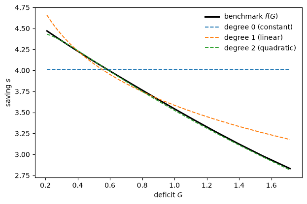
Fig. 86.2 Parameterized expectations rules of increasing degree#
The constant family cannot represent a saving rule that depends on the deficit at all, so the best it can do is a flat line through the middle of the data.
That flat line is an approximate equilibrium — a fixed point of the learning scheme — but it satisfies the first-order condition only on average, not state by state.
The linear family does much better but bends the wrong way at the extremes.
The quadratic family is visually indistinguishable from the benchmark: because the true \(f(G)\) is very nearly quadratic here, a three-parameter rule essentially nails it.
We can quantify “how close” two ways: by the distance to the benchmark, and by the residual in the first-order condition under the true kernel, the honest measure of how far an approximate equilibrium is from an exact one.
rows = []
for deg in (0, 1, 2):
    s_hat = rules[deg]
    sup = np.max(np.abs(s_hat - s_benchmark))
    rms = np.sqrt(ergodic @ (s_hat - s_benchmark)**2)
    rows.append([labels[deg], sup, rms, foc_residual(s_hat)])

pd.DataFrame(rows, columns=["family", "sup $|s - f|$",
                            "ergodic RMS", "FOC residual"]).set_index("family").round(4)
| sup $|s - f|$ | ergodic RMS | FOC residual | |
|---|---|---|---|
| family | |||
| degree 0 (constant) | 1.1826 | 0.3230 | 0.0090 |
| degree 1 (linear) | 0.3458 | 0.0671 | 0.0039 |
| degree 2 (quadratic) | 0.0386 | 0.0110 | 0.0006 |
Every column falls as the family grows richer.
The first-order-condition residual — the quantity that is exactly zero at a rational expectations equilibrium and positive at an approximate one — drops by more than an order of magnitude from the constant family to the quadratic.
Note
Richer is not always better with finite data.
Push the degree higher and the extra terms start chasing sampling noise in the tails of the deficit distribution, where observations are scarce, and the sup-norm error can tick back up even as the fit improves where agents actually spend their time.
That is the same phenomenon as the slowly-learned rare state in Adaptive Agents in an Overlapping Generations Monetary Economy, seen from the approximation side: a scheme fits well where the data is, and the cost of misfitting a rarely-visited region is small in terms of expected utility.
Exercise 86.1 explores this.
86.5. Learning is equilibrium computation#
So far parameterized expectations is an algorithm we run to compute an equilibrium.
Now comes the point of the whole lecture.
Write the same algorithm recursively — updating \(\theta\) once per period as a single new observation arrives, rather than re-regressing a whole simulated panel — and it becomes a model of adaptive agents learning in real time.
The recursive form is ordinary recursive least squares:
where \(y_t\) is the same realized regressand as before and \(R_t\) tracks the second moment of the regressors.
This is the identical object we met in Adaptive Agents in an Overlapping Generations Monetary Economy: a stochastic-approximation recursion with a \(1/t\) gain.
The only difference from the state-by-state learning there is that \(\theta\) indexes a parametric rule, so a single observation updates the saving rule everywhere at once.
def online_pea(degree=2, T=500_000, seed=0, ridge=1e-3):
    """
    Recursive-least-squares parameterized expectations: the learning economy.

    Young agents at t save according to the current θ; next period the Euler
    equation's realized value arrives and θ is updated once.  Returns the θ
    path and the final implied saving rule.
    """
    G_sim = simulate_deficit(T, seed)
    θ = np.array([2.0] + [0.0] * degree)
    R = ridge * np.eye(degree + 1)

    def saving(g, θ):
        ψ = np.clip(basis(np.array([g]), degree)[0] @ θ, 0.05, 50)
        return np.clip(s_from_psi(ψ), g + 0.05, w1 - 0.05)

    x_prev = None
    θ_path = np.empty((T, degree + 1))
    for t in range(T):
        s_t = saving(G_sim[t], θ)
        if x_prev is not None:                                  # date t-1 Euler realizes now
            y = (s_t - G_sim[t]) / (w2 + (s_t - G_sim[t]))
            gain = 1.0 / (t + 1)
            R += gain * (np.outer(x_prev, x_prev) - R)
            θ = θ + gain * np.linalg.solve(R, x_prev * (y - x_prev @ θ))
        x_prev = basis(np.array([G_sim[t]]), degree)[0]
        θ_path[t] = θ

    s_grid = np.array([saving(g, θ) for g in G])
    return θ_path, s_grid


θ_path, s_online = online_pea()
print(f"online PEA: sup error = {np.max(np.abs(s_online - s_benchmark)):.4f},  "
      f"ergodic RMS = {np.sqrt(ergodic @ (s_online - s_benchmark)**2):.4f}")
online PEA: sup error = 0.0837, ergodic RMS = 0.0480
fig, axes = plt.subplots(1, 2, figsize=(11, 4.2))

axes[0].plot(θ_path[:, 0], label=r"$\theta_0$", lw=2)
axes[0].plot(θ_path[:, 1], label=r"$\theta_1$", lw=2)
axes[0].plot(θ_path[:, 2], label=r"$\theta_2$", lw=2)
axes[0].set_xscale('log')
axes[0].set_xlabel("$t$  (log scale)")
axes[0].set_ylabel(r"$\theta_t$")
axes[0].set_title("coefficients learned in real time")
axes[0].legend(frameon=False, fontsize=9)

axes[1].plot(G, s_benchmark, 'k-', lw=2.2, label="benchmark $f(G)$")
axes[1].plot(G, s_online, 'C3--', lw=1.5, label="online PEA")
axes[1].set_xlabel("deficit $G$")
axes[1].set_ylabel("saving $s$")
axes[1].set_title("saving rule after learning")
axes[1].legend(frameon=False)
plt.tight_layout()
plt.show()
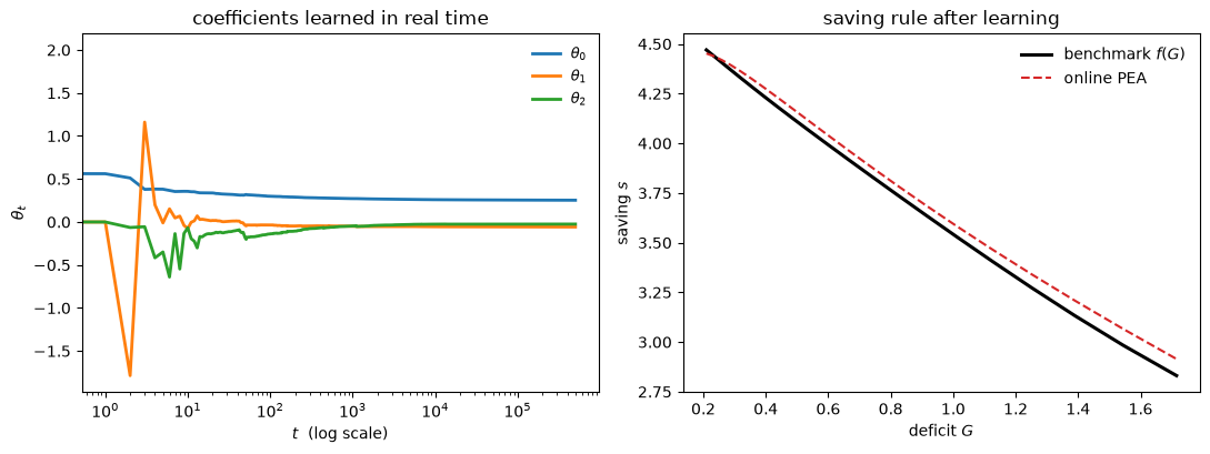
Fig. 86.3 Online learning of the saving rule#
The coefficients settle down, and the saving rule they imply tracks the benchmark closely.
The small remaining gap is the signature of a scheme that has not quite finished converging.
Convergence is slow: the \(1/t\) gain guarantees it but does not hurry it, and the online scheme takes hundreds of thousands of periods to reach an accuracy the batch algorithm attains in a handful of passes.
That gap is exactly the difference between an agent constrained to learn from experience as it arrives and a modeller free to re-use a whole simulated history at once.
But the limit is the same object.
Sargent’s summary:
Learning algorithms and equilibrium computation algorithms look like each other. Equilibrium computation algorithms often have interpretations as centralized learning algorithms whereby the model builder, acting in a role of ‘social planner,’ gropes for a set of pricing functions for markets and decision rules for agents that will satisfy all of the individual optimum conditions and market-clearing conditions. We have also seen that learning systems with boundedly rational agents sometimes have interpretations as decentralized equilibrium computation algorithms.
This is why Marcet arrived at parameterized expectations as a computational method by way of earlier work on the dynamics of least squares learning.
The two are the same recursion read in two directions.
86.6. Learning without a functional form#
The parametric route is fast but stakes everything on the family.
If no member of \(\{f(\cdot, \theta)\}\) supports an equilibrium, the scheme converges to an approximate equilibrium and stops.
The non-parametric alternative imposes no functional form.
Following the recursive kernel estimators of Chen and White [1998], an agent estimates the conditional expectation \(\psi(G)\) directly from a kernel-weighted average of past realized values, letting the data choose the shape.
The recursive kernel density estimator is itself a stochastic-approximation recursion,
with a bandwidth \(h_t \searrow 0\), the same \(1/t\)-gain shape as everything else in this lecture, now updating an entire estimated density rather than a finite parameter vector.
What we implement below is the batch counterpart of that recursion: a Nadaraya–Watson estimate of \(\psi(G)\), formed as a kernel-weighted average of the realized regressand \(y\) over a whole simulated history, with weights that fall off with distance in \(\log G\), and iterated to a fixed point.
Reading it in batch form keeps the comparison clean, because the parametric scheme we are measuring it against is also in batch form.
The recursive display above stands to this smoother exactly as (86.3) stands to the batch algorithm of the previous section: same estimator, read as a real-time learning rule rather than as a computation.
def kernel_smoother(T=400_000, seed=0, h=0.06, n_iter=40, damp=0.5):
    """
    Non-parametric parameterized expectations.  ψ(G) is estimated by a
    Nadaraya-Watson smoother of the realized regressand -- no functional form.
    The rule is iterated to a self-consistent fixed point.
    """
    G_sim = simulate_deficit(T, seed)
    log_sim = np.log(G_sim[:-1])
    # kernel weights of each grid point against the whole simulated history
    W = np.array([np.exp(-0.5 * ((np.log(g) - log_sim) / h)**2) for g in G])
    W /= W.sum(axis=1, keepdims=True)

    s_grid = np.full(len(G), (w1 - w2) / 2)
    for _ in range(n_iter):
        s = np.clip(np.interp(np.log(G_sim), np.log(G), s_grid), G_sim + 0.05, w1 - 0.05)
        y = (s[1:] - G_sim[1:]) / (w2 + (s[1:] - G_sim[1:]))
        ψ = W @ y
        s_new = np.clip(s_from_psi(ψ), G + 0.05, w1 - 0.05)
        if np.max(np.abs(s_new - s_grid)) < 1e-8:
            s_grid = s_new
            break
        s_grid = damp * s_new + (1 - damp) * s_grid
    return s_grid


s_kernel = kernel_smoother()
print(f"kernel smoother: sup error = {np.max(np.abs(s_kernel - s_benchmark)):.4f},  "
      f"ergodic RMS = {np.sqrt(ergodic @ (s_kernel - s_benchmark)**2):.4f}")
kernel smoother: sup error = 0.0816, ergodic RMS = 0.0166
fig, ax = plt.subplots(figsize=(6.5, 4.2))
ax.plot(G, s_benchmark, 'k-', lw=2.2, label="benchmark $f(G)$")
ax.plot(G, s_kernel, 'C3o', ms=4, label="kernel smoother")
ax.set_xlabel("deficit $G$")
ax.set_ylabel("saving $s$")
ax.legend(frameon=False)
plt.show()
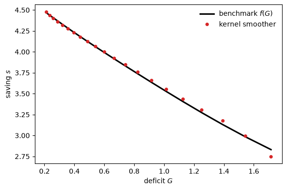
Fig. 86.4 Kernel smoother approximation to the saving rule#
With no functional form imposed, the kernel learner recovers the benchmark to about the same accuracy as the quadratic parametric rule.
That the two do equally well here is not a coincidence to lean on.
It is because the true \(f(G)\) happens to be almost exactly quadratic, so the parametric family we chose was very nearly correct.
When it is not, the two part ways, and the trade-off is the one familiar from econometrics:
the parametric scheme learns fast and extrapolates gracefully, but is only as good as its family; a poorly chosen family delivers an approximate equilibrium and no warning;
the non-parametric scheme cannot be led astray by a bad functional form, but pays for its flexibility with slower learning and with bias where the data is thin, at the edges of the deficit’s range, where the kernel has few neighbours to average.
Both are recursions of the same shape.
Which one an adaptive agent should use is, once again, one of the modelling choices that the bounded-rationality program forces into the open and that rational expectations quietly made for us.
86.7. Concluding remarks#
The overlapping generations model gave us a clean laboratory for a general lesson.
An adaptive agent in an environment with a large or continuous state cannot learn a separate response for every contingency.
It must generalize, imposing some structure that lets a finite amount of experience inform behavior across the whole state space.
Whether that structure is a low-order polynomial, a kernel bandwidth, or something else is a modelling choice with real consequences: it fixes whether the achievable limit is a rational expectations equilibrium or merely an approximation to one.
That same act of generalization is what makes learning and equilibrium computation two faces of one object.
Marcet’s algorithm computes an equilibrium by parameterizing an expectation and regressing; an adaptive agent learns by parameterizing an expectation and regressing; the recursions coincide.
The next lecture, Money as a Medium of Exchange among Artificially Intelligent Agents, carries the generalization problem to its sharpest form.
There the state and action spaces are large enough that enumerating rules is out of the question, and agents must discover a compact set of good rules from scratch, using John Holland’s classifier systems and genetic algorithm in place of the least squares and kernel machinery of this lecture.
86.8. Exercises#
Exercise 86.1
The note above claimed that pushing the polynomial degree too high can hurt the sup-norm fit, because high-order terms chase sampling noise in the sparsely-visited tails of the deficit distribution.
Verify it.
Run the batch parameterized-expectations algorithm for degrees \(0\) through \(5\) and report two error measures against the benchmark: the sup norm over the whole grid, and the RMS error weighted by the ergodic distribution of the deficit (i.e. weighted by where agents actually operate).
Which measure is monotone in the degree, and which is not?
Interpret.
Solution
rows = []
for deg in range(6):
    s_hat = parameterized_expectations(deg, T=150_000)
    sup = np.max(np.abs(s_hat - s_benchmark))
    rms = np.sqrt(ergodic @ (s_hat - s_benchmark)**2)
    rows.append([deg, sup, rms])

pd.DataFrame(rows, columns=["degree", "sup error (whole grid)",
                            "ergodic RMS (where agents live)"]).set_index("degree").round(4)
| sup error (whole grid) | ergodic RMS (where agents live) | |
|---|---|---|
| degree | ||
| 0 | 1.1880 | 0.3243 |
| 1 | 0.3505 | 0.0677 |
| 2 | 0.0472 | 0.0128 |
| 3 | 0.1561 | 0.0203 |
| 4 | 0.1854 | 0.0221 |
| 5 | 0.2201 | 0.0241 |
The ergodic-weighted error falls monotonically and then flattens: once the family is rich enough to capture the curvature of \(f\) where the deficit actually spends its time, extra terms add nothing.
The sup-norm error falls at first but then rises again.
The high-order polynomials fit the center well but oscillate at the ends of the grid, where the ergodic distribution puts almost no mass and so the regression has almost no data to discipline them.
This is the approximation-side image of the rare-state problem from Adaptive Agents in an Overlapping Generations Monetary Economy.
A learning scheme allocates its accuracy to where the observations are.
Misfitting a rarely-visited region shows up starkly in the sup norm but costs almost nothing in expected utility, which is why the ergodic-weighted measure is the economically relevant one.
Exercise 86.2
The constant family (degree 0) delivers an approximate equilibrium: a single saving rate, independent of the deficit, that satisfies the first-order condition only on average.
There is a natural benchmark for it.
Compute the single saving rate \(\bar s\) that a degree-0 parameterized-expectations agent converges to, and compare it with the saving rate of the economy in which the deficit is fixed forever at its mean \(\bar G\).
Are they the same?
Should they be?
Solution
# the degree-0 approximate equilibrium
s_const = parameterized_expectations(0)[0]        # constant across states

# the deterministic economy with G fixed at its mean.  Like the constant-deficit
# model of the previous lecture it has two steady states; we take the high-saving
# (low-inflation) one, found by iterating the saving map to its stable fixed point.
G_mean = ergodic @ G

def deterministic_saving(G_fixed, damp=0.5):
    s = (w1 - w2) / 2
    for _ in range(1000):
        ψ = (s - G_fixed) / (w2 + (s - G_fixed))
        s = damp * s + (1 - damp) * s_from_psi(ψ)
    return s

s_fixed = deterministic_saving(G_mean)

print(f"degree-0 approximate-equilibrium saving rate : {s_const:.4f}")
print(f"mean deficit  E[G]                           : {G_mean:.4f}")
print(f"saving in the economy with G fixed at E[G]   : {s_fixed:.4f}")
degree-0 approximate-equilibrium saving rate : 4.0137
mean deficit  E[G]                           : 0.6537
saving in the economy with G fixed at E[G]   : 4.0327
They are close but not equal.
The degree-0 agent picks the single saving rate that best fits the first-order condition across the stochastic economy, an average over the realized distribution of returns.
The fixed-deficit economy replaces that whole distribution with a single degenerate one at the mean deficit.
By a Jensen-type argument these need not coincide: the first-order condition is nonlinear in the return, so its expectation over a spread-out distribution of deficits differs from its value at the mean deficit.
They would agree only if the deficit were deterministic to begin with.
The lesson is that an approximate equilibrium is not a naive “certainty-equivalent” object.
Even the crudest one-parameter learner is responding to the whole distribution of outcomes it experiences, not to a point forecast.
Exercise 86.3
The non-parametric kernel learner has one free tuning constant: the bandwidth \(h\).
Explore its effect.
Run the kernel learner for a range of bandwidths and report the sup and ergodic-weighted errors against the benchmark.
Explain the shape of the trade-off, and relate the two failure modes to the bias–variance decomposition.
Solution
rows = []
for h in (0.03, 0.05, 0.08, 0.12, 0.20):
    s_h = kernel_smoother(h=h)
    sup = np.max(np.abs(s_h - s_benchmark))
    rms = np.sqrt(ergodic @ (s_h - s_benchmark)**2)
    rows.append([h, sup, rms])

table = pd.DataFrame(rows, columns=["bandwidth $h$", "sup error",
                                    "ergodic RMS"]).set_index("bandwidth $h$")
table.round(4)
| sup error | ergodic RMS | |
|---|---|---|
| bandwidth $h$ | ||
| 0.03 | 0.2140 | 0.0197 |
| 0.05 | 0.1269 | 0.0148 |
| 0.08 | 0.0873 | 0.0282 |
| 0.12 | 0.2045 | 0.0626 |
| 0.20 | 0.5110 | 0.1312 |
fig, ax = plt.subplots(figsize=(7, 4.2))
for h, colour in [(0.03, 'C0'), (0.08, 'C1'), (0.20, 'C2')]:
    ax.plot(G, kernel_smoother(h=h), 'o-', ms=3, lw=0.8, color=colour, label=f"$h = {h}$")
ax.plot(G, s_benchmark, 'k-', lw=2, label="benchmark")
ax.set_xlabel("deficit $G$")
ax.set_ylabel("saving $s$")
ax.legend(frameon=False)
plt.show()
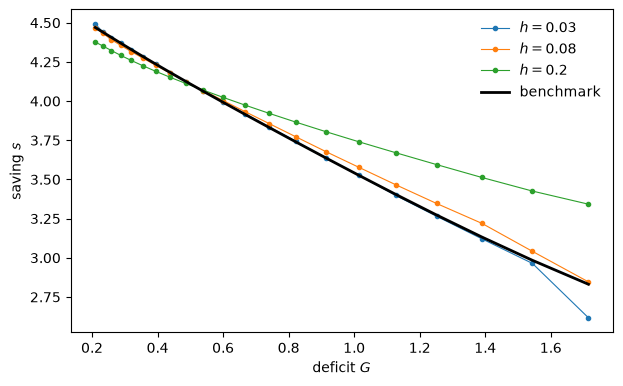
There is an interior optimum.
A small bandwidth averages over few neighbours, so the estimate is noisy: it wiggles around the benchmark, and the wiggle is worst at the edges where neighbours are scarce.
This is the variance end of the trade-off.
A large bandwidth averages over a wide window, smoothing the estimate but flattening the genuine curvature of \(f(G)\), so the rule is pulled toward a straight line.
This is the bias end.
The bandwidth is the non-parametric counterpart of the polynomial degree in Exercise 86.1: both control how much structure the learner imposes, and both have a sweet spot that trades misfit-from-too-little-flexibility against noise-from-too-much.
The bounded-rationality program does not tell us where that spot is; it is one more choice that replaces the single discipline of rational expectations with a menu of plausible alternatives.