88. Genetic Algorithms and Classifier Systems#
88.1. Overview#
The lectures so far gave adaptive agents a fairly econometric brain.
In Adaptive Agents in an Overlapping Generations Monetary Economy and Learning, Approximation, and Equilibrium Computation they ran recursive least squares; in Exchange Rate Indeterminacy, Learning, and Experiments they took Newton steps against realized utility.
In each case an agent held a parametric rule and tuned its coefficients.
This lecture surveys a different toolbox, the one Sargent [1993] draws from John Holland’s work on artificial intelligence and from the connectionist literature on neural networks.
These devices do not tune the coefficients of a fixed rule.
They discover the rule itself, out of a large space of possibilities, from experience.
Sargent’s framing is that the bounded-rationality program asks us to populate models with agents who “behave like econometricians,” and that the artificial-intelligence literature is a catalogue of candidate brains for them:
It is from the store of methods built up in these literatures that we shall select the ‘brains’ to give our boundedly rational agents.
We tour four of them:
the perceptron, the simplest neural network, which turns out to be a linear discriminant function, a direct link to the “agents as econometricians” reading;
the Hopfield network, an associative memory that recovers stored patterns from corrupted inputs by rolling downhill on an energy function;
the genetic algorithm, Holland’s population-based search, which we set loose on Axelrod’s iterated prisoner’s dilemma and watch discover cooperation;
the classifier system, Holland’s “brain as a competitive economy” of if-then rules, whose simplest instance — a two-armed bandit — already exposes a subtle limitation.
We close with evolutionary programming: the idea that a population of adaptive agents, plodding toward an equilibrium, can be used to compute equilibria that we cannot solve for directly.
That is the idea Money as a Medium of Exchange among Artificially Intelligent Agents carries out in full, so this lecture is the machinery on which the next one is built.
Let’s start with some imports.
import numpy as np
import matplotlib.pyplot as plt
88.2. The perceptron: an agent as a discriminant function#
The simplest neural network is a single perceptron: \(k\) inputs \(x_i\), weights \(w_i\), and one output
where \(S\) is a “squasher” mapping \(\mathbb{R}\) onto \([0, 1]\): a step function, or the sigmoid \(S(z) = 1/(1 + e^{-z})\), or any cumulative distribution function.
For fixed weights the perceptron is a classifier: it fires (\(y = 1\)) when \(w^\top x > 0\) and stays quiet otherwise, so the boundary \(w^\top x = 0\) is a hyperplane separating two classes.
Training the perceptron — choosing \(w\) to minimize \(\sum_t (y_t - S(w^\top x_t))^2\) — is a nonlinear least squares problem, solved by the familiar stochastic-gradient recursion
which is the same \(1/t\)-flavored update that ran the learning models of the previous lectures.
Take the book’s example: separate football players from economists on two standardized features.
rng = np.random.default_rng(0)
n = 100
economists = rng.multivariate_normal([-1.0, -0.3], [[0.5, 0.1], [0.1, 0.5]], n)
players    = rng.multivariate_normal([1.2,  0.8], [[0.6, 0.0], [0.0, 0.6]], n)
X = np.vstack([economists, players])
y = np.r_[np.zeros(n), np.ones(n)]
X_aug = np.column_stack([np.ones(len(X)), X])          # prepend an intercept

def sigmoid(z):
    return 1 / (1 + np.exp(-z))

w = np.zeros(3)
for _ in range(200):                                    # train by stochastic gradient
    for t in rng.permutation(len(X)):
        w += 0.1 * (y[t] - sigmoid(X_aug[t] @ w)) * X_aug[t]

print(f"training accuracy: {np.mean((sigmoid(X_aug @ w) > 0.5) == y):.3f}")
training accuracy: 0.930
The point Sargent [1993] stresses is that this is nothing exotic to an econometrician: the perceptron’s decision boundary is essentially a linear discriminant function.
Compare the perceptron’s boundary normal to Fisher’s linear discriminant direction.
m0, m1 = X[y == 0].mean(0), X[y == 1].mean(0)
S_within = np.cov(X[y == 0].T) * n + np.cov(X[y == 1].T) * n
lda_direction = np.linalg.solve(S_within, m1 - m0)
lda_direction /= np.linalg.norm(lda_direction)
perceptron_direction = w[1:] / np.linalg.norm(w[1:])

print(f"perceptron boundary normal : {perceptron_direction.round(3)}")
print(f"Fisher discriminant direction: {lda_direction.round(3)}")
print(f"cosine similarity: {abs(perceptron_direction @ lda_direction):.4f}")
perceptron boundary normal : [0.946 0.324]
Fisher discriminant direction: [0.925 0.38 ]
cosine similarity: 0.9982
fig, ax = plt.subplots(figsize=(6.5, 5))
ax.scatter(*economists.T, s=18, c='C0', label="economists ($y=0$)")
ax.scatter(*players.T, s=18, c='C1', label="football players ($y=1$)")
xs = np.linspace(X[:, 0].min(), X[:, 0].max(), 2)
ax.plot(xs, -(w[0] + w[1]*xs) / w[2], 'k-', lw=1.5, label="perceptron boundary")
ax.set_xlabel("weight (standardized)")
ax.set_ylabel("salary (standardized)")
ax.legend(frameon=False)
plt.show()
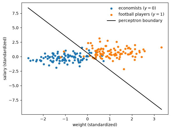
Fig. 88.1 Perceptron boundary separating the two groups#
The two directions are all but identical.
Minsky and Papert’s famous critique [Minsky and Papert, 1969] was precisely that a single perceptron can represent only a linear discriminant, and so cannot separate classes that a line cannot.
The revival of the field came with the recognition that layering perceptrons — feeding their outputs into further perceptrons — approximates any nonlinear discriminant, the subject of Introduction to Artificial Neural Networks.
For our purposes the perceptron is the entry in the catalogue closest to what the previous lectures already did: a parametric rule, trained by gradient descent, that an econometrician would recognize on sight.
The remaining three brains are stranger.
88.3. Associative memory: the Hopfield network#
The second device stores patterns and recalls them from corrupted fragments.
Represent a pattern as a vector of \(\pm 1\) of length \(N\).
We want to store \(p\) patterns \(\sigma^1, \ldots, \sigma^p\) so that each is a fixed point of a dynamical system, and so that feeding in a corrupted version converges quickly to the nearest stored pattern.
The Hopfield network does this with the dynamics
and a weight matrix built from the patterns themselves.
When the patterns are orthogonal, Hebb’s rule \(w = \tfrac{1}{N}\sigma\sigma^\top\) suffices; for merely linearly independent (correlated) patterns one uses the projection rule \(w = \tfrac{1}{N}\sigma V^{-1}\sigma^\top\) with \(V = \tfrac{1}{N}\sigma^\top \sigma\).
Both make each stored pattern an exact fixed point.
We store five letters on a \(5\times5\) pixel grid, and because letters share many pixels, they are correlated, so the projection rule is the right one.
PATTERNS = {
    'A': ["01110", "10001", "11111", "10001", "10001"],
    'E': ["11111", "10000", "11110", "10000", "11111"],
    'I': ["11111", "00100", "00100", "00100", "11111"],
    'O': ["01110", "10001", "10001", "10001", "01110"],
    'T': ["11111", "00100", "00100", "00100", "00100"],
}

def to_vector(rows):
    return np.array([1 if c == '1' else -1 for r in rows for c in r])

letters = list(PATTERNS)
σ = np.array([to_vector(PATTERNS[c]) for c in letters])      # (p, N)

def projection_rule(patterns):
    "Weight matrix making each (correlated) pattern an exact fixed point."
    N = patterns.shape[1]
    Σ = patterns.T                                          # (N, p)
    V = Σ.T @ Σ / N
    return Σ @ np.linalg.inv(V) @ Σ.T / N

def energy(w, s):
    "Hopfield energy; stored patterns are local minima."
    return -0.5 * s @ w @ s

def recall(w, s0, max_iter=30):
    "Iterate sgn(w s) to a fixed point."
    s = s0.copy()
    for _ in range(max_iter):
        s_new = np.sign(w @ s)
        s_new[s_new == 0] = 1
        if np.array_equal(s_new, s):
            break
        s = s_new
    return s

w_hop = projection_rule(σ)
fixed = all(np.array_equal(np.sign(w_hop @ σ[i]), σ[i]) for i in range(len(letters)))
print(f"all stored letters are fixed points: {fixed}")
print(f"energy of each stored letter: {[round(energy(w_hop, σ[i]), 1) for i in range(len(letters))]}")
all stored letters are fixed points: True
energy of each stored letter: [np.float64(-12.5), np.float64(-12.5), np.float64(-12.5), np.float64(-12.5), np.float64(-12.5)]
Every stored letter sits at the same energy \(-N/2\) and is a fixed point.
Now corrupt a few pixels and let the network fall back to the nearest memory.
rng = np.random.default_rng(3)
show = ['E', 'O', 'T']

fig, axes = plt.subplots(len(show), 3, figsize=(6, 6))
for row, letter in enumerate(show):
    i = letters.index(letter)
    corrupt = σ[i].copy()
    corrupt[rng.choice(25, 4, replace=False)] *= -1             # flip 4 pixels
    recovered = recall(w_hop, corrupt)
    for col, (img, title) in enumerate([(σ[i], "stored"),
                                        (corrupt, "corrupted"),
                                        (recovered, "recovered")]):
        axes[row, col].imshow(img.reshape(5, 5), cmap='binary', vmin=-1, vmax=1)
        axes[row, col].set_xticks([])
        axes[row, col].set_yticks([])
        if row == 0:
            axes[row, col].set_title(title)
plt.tight_layout()
plt.show()
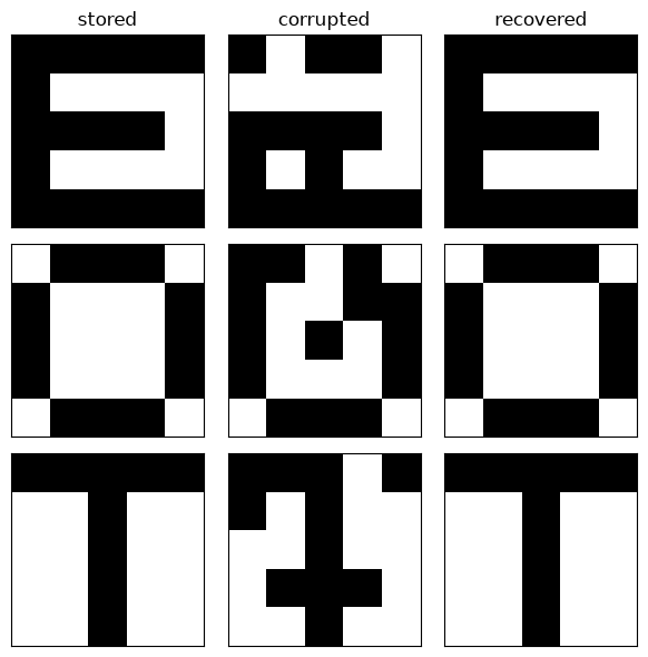
Fig. 88.2 Hopfield recall of letters from corrupted inputs#
The corrupted letters snap back to their originals.
How reliably depends on how much is corrupted and on how correlated the patterns are.
A corrupted letter can occasionally land in a different letter’s basin, or in a spurious mixture the designer never stored.
for n_flip in (3, 5, 7):
    correct = 0
    for i in range(len(letters)):
        for _ in range(40):
            corrupt = σ[i].copy()
            corrupt[rng.choice(25, n_flip, replace=False)] *= -1
            if np.array_equal(recall(w_hop, corrupt), σ[i]):
                correct += 1
    print(f"{n_flip} pixels flipped: recovered exactly {correct}/{len(letters)*40}")
3 pixels flipped: recovered exactly 179/200
5 pixels flipped: recovered exactly 138/200
7 pixels flipped: recovered exactly 77/200
The mechanism is worth naming because it recurs throughout this program.
Recall is descent on an energy function whose local minima are the stored patterns.
Feeding in a corrupted pattern places the system on the energy surface near the right minimum, and the dynamics roll it down.
This is exactly the geometry behind simulated annealing, the method the book invokes for escaping unwanted local minima: add a controlled amount of random “shaking,” large at first and declining over time, so the system can hop out of shallow spurious basins before settling into a deep one.
It is the stochastic cousin of Newton’s method, and it reappears as the “genetic” experimentation in classifier systems.
88.4. The genetic algorithm#
The third brain does not descend a smooth surface at all.
Holland’s genetic algorithm searches “rugged landscapes” that lack the smoothness Newton’s method needs, by evolving a population of candidate solutions encoded as binary strings.
Given a fitness function \(f\) to maximize, and a population of \(N\) strings of length \(S\), one generation applies four operators:
Evaluation: compute each string’s fitness \(f(x_i)\).
Reproduction: copy strings into the next generation with probability proportional to fitness (a “biased roulette wheel”).
Crossover: pair strings up and swap their tails at a random cut point, forming children that recombine their parents’ segments.
Mutation: flip each bit independently with a small probability \(p_m\).
Reproduction concentrates the population on what already works; crossover and mutation inject new candidates.
Crossover is the workhorse: it “preserves long sections of genetic structure” — Holland’s schemata — while still exploring, provided the population is diverse enough to recombine.
Crucially, the individual strings do not learn: each lives one generation and dies.
Only the society, the sequence of populations, learns.
That is what makes the genetic algorithm awkward as a model of one brain, and a better fit as a model of a population or a market, a point that matters when we reach Money as a Medium of Exchange among Artificially Intelligent Agents.
88.4.1. Axelrod’s iterated prisoner’s dilemma#
Axelrod [1987] used the genetic algorithm to evolve strategies for the iterated prisoner’s dilemma, the game whose round-robin tournament, famously, was won by tit-for-tat.
Two players each choose to Cooperate or Defect; the payoffs reward defection against a cooperator but punish mutual defection.
# 1 = Cooperate, 0 = Defect;  T > R > P > S is the prisoner's dilemma ranking
T_pay, R_pay, P_pay, S_pay = 5, 3, 1, 0

def payoff(a, b):
    "My payoff when I play a against opponent's b."
    if a and b:       return R_pay        # both cooperate
    if not a and not b: return P_pay      # both defect
    if not a and b:   return T_pay        # I defect, they cooperate
    return S_pay                          # I cooperate, they defect
Following Axelrod, a strategy is a 70-bit string: a strategy conditions on the outcomes of the last three rounds.
Each round is one of four outcomes (my move, opponent’s move), so three rounds give \(4^3 = 64\) possible histories, and 64 bits specify the action in each.
The remaining 6 bits encode a presumed pre-game history to get the first moves going.
def play(gene, opponent, n_rounds=150):
    "Play a 70-bit genetic strategy against an opponent; return average payoffs."
    action, premise = gene[:64], gene[64:]
    hist = list(premise)                     # last 3 rounds as [my, opp] pairs
    my_moves, opp_moves = [], []
    my_total = opp_total = 0
    for t in range(n_rounds):
        idx = 0
        for bit in hist:
            idx = (idx << 1) | bit           # 6 history bits -> index 0..63
        a = action[idx]                      # my move from the lookup table
        b = opponent(my_moves, opp_moves, t)
        my_total += payoff(a, b)
        opp_total += payoff(b, a)
        my_moves.append(a)
        opp_moves.append(b)
        hist = [a, b] + hist[:4]             # roll the 3-round window
    return my_total / n_rounds, opp_total / n_rounds
The strategy is bred to do well against a fixed panel of opponents.
Each panel member is a function of the histories as that member sees them: its first argument is what its opponent has played and its second is what it has played itself.
panel_rng = np.random.default_rng(2024)

def all_cooperate(opp_moves, own_moves, t): return 1
def all_defect(opp_moves, own_moves, t):    return 0
def tit_for_tat(opp_moves, own_moves, t):   return 1 if t == 0 else opp_moves[-1]
def grudger(opp_moves, own_moves, t):       return 0 if 0 in opp_moves else 1
def random_play(opp_moves, own_moves, t):   return int(panel_rng.random() < 0.5)

PANEL = {'AllC': all_cooperate, 'AllD': all_defect, 'TFT': tit_for_tat,
         'Grudger': grudger, 'Random': random_play}

def fitness(gene):
    "Average payoff against the whole panel."
    return np.mean([play(gene, opp)[0] for opp in PANEL.values()])
Tit-for-tat copies what its opponent last did, and the grudger defects forever once its opponent has defected once.
Now evolve.
def evolve(N=60, generations=80, p_mut=0.01, seed=0):
    rng = np.random.default_rng(seed)
    pop = rng.integers(0, 2, (N, 70))
    best_hist, mean_hist = [], []
    for _ in range(generations):
        fit = np.array([fitness(pop[i]) for i in range(N)])
        best_hist.append(fit.max())
        mean_hist.append(fit.mean())
        weight = fit - fit.min() + 1e-6                    # shift positive for roulette
        nxt = np.empty_like(pop)
        for k in range(0, N, 2):
            i, j = np.searchsorted(np.cumsum(weight), rng.random(2) * weight.sum())
            cut = rng.integers(1, 70)                      # single-point crossover
            c1 = np.concatenate([pop[i, :cut], pop[j, cut:]])
            c2 = np.concatenate([pop[j, :cut], pop[i, cut:]])
            for c in (c1, c2):
                c[rng.random(70) < p_mut] ^= 1             # mutation
            nxt[k], nxt[k+1] = c1, c2
        pop = nxt
    fit = np.array([fitness(pop[i]) for i in range(N)])
    return pop[fit.argmax()], np.array(best_hist), np.array(mean_hist)


panel_rng = np.random.default_rng(0)     # reset the panel's randomizer
champion, best_hist, mean_hist = evolve()
print(f"generation 0: best fitness {best_hist[0]:.3f}")
print(f"generation {len(best_hist)-1}: best fitness {best_hist[-1]:.3f}")
generation 0: best fitness 2.504
generation 79: best fitness 2.672
fig, ax = plt.subplots(figsize=(7.5, 4))
ax.plot(best_hist, label="best in population", lw=2)
ax.plot(mean_hist, label="population mean", lw=2)
ax.set_xlabel("generation")
ax.set_ylabel("panel fitness")
ax.legend(frameon=False)
plt.show()
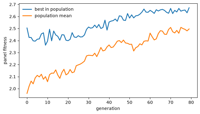
Fig. 88.3 Population fitness across generations#
Fitness climbs, then holds.
What kind of strategy did evolution find?
print("evolved champion's average payoff against each opponent:")
for name, opp in PANEL.items():
    me, them = play(champion, opp)
    print(f"  vs {name:8s}:  me = {me:.2f},  opponent = {them:.2f}")
evolved champion's average payoff against each opponent:
  vs AllC    :  me = 5.00,  opponent = 0.00
  vs AllD    :  me = 1.00,  opponent = 1.00
  vs TFT     :  me = 2.98,  opponent = 2.98
  vs Grudger :  me = 1.01,  opponent = 1.07
  vs Random  :  me = 2.80,  opponent = 1.33
The evolved strategy is nice and retaliatory, in Axelrod’s language.
It reaches mutual cooperation with the cooperative opponents (AllC, TFT, Grudger), refuses to be suckered by AllD (settling into mutual defection near the punishment payoff), and exploits Random.
Nobody told it to cooperate; cooperation emerged because it pays against a panel that contains cooperators.
And it does all this better than tit-for-tat itself would against the same panel.
def play_function(strategy, opponent, n=150):
    "Average payoff of a stateful strategy function against an opponent."
    mine, theirs, total = [], [], 0
    for t in range(n):
        # each side is passed its opponent's history first, then its own
        a, b = strategy(theirs, mine, t), opponent(mine, theirs, t)
        total += payoff(a, b)
        mine.append(a)
        theirs.append(b)
    return total / n

panel_rng = np.random.default_rng(0)
tft_fitness = np.mean([play_function(tit_for_tat, opp) for opp in PANEL.values()])
print(f"tit-for-tat's own panel fitness:  {tft_fitness:.3f}")
print(f"evolved champion's panel fitness: {best_hist[-1]:.3f}")
tit-for-tat's own panel fitness:  2.432
evolved champion's panel fitness: 2.672
This reproduces Axelrod’s headline finding: the genetic algorithm “produced a strategy that would have won the tournament, and in particular would have outplayed the ‘tit-for-tat’ strategy that won the tournament.”
It behaves much like tit-for-tat against cooperators, but its extra memory lets it squeeze more out of exploitable opponents that tit-for-tat leaves alone.
The margin is not large, and it should not be.
Tit-for-tat is a strong strategy against this panel; what the extra memory buys is a modest edge against the opponents that tit-for-tat handles adequately but not optimally.
88.5. Classifier systems#
The genetic algorithm evolves a population in which no individual learns.
Holland’s classifier system puts the same evolutionary machinery inside a single agent, as a model of one brain.
Sargent describes it as Holland’s vision of the mind as a competitive economy:
The statements compete with one another for the opportunity to decide. The classifier system incorporates elements of the genetic algorithm with other aspects in a way that represents a brain in terms that Holland describes as a competitive economy.
A classifier system has:
Classifiers, if-then rules encoded as strings over the trinary alphabet \(\{0, 1, \#\}\) whose condition part matches states and whose action part prescribes a move, with \(\#\) a wildcard (“I don’t care”) that lets general rules coexist with specific ones.
A decoder that, given the current state, finds which classifiers’ conditions match.
An auction that selects one matching classifier to act: the strongest, or one chosen with probability proportional to strength.
An accounting system that updates each classifier’s strength — a running average of the net rewards its decisions earn — and, in sequential problems, passes reward backward from rules that collect payoffs to the rules that set them up.
Genetic operators that create new classifiers, generalize (add \(\#\)’s) and specialize (remove them), so the system’s very vocabulary evolves.
88.5.1. A two-armed bandit#
The simplest classifier system, due to Brian Arthur and Carl Simon, plays a two-armed bandit.
Arm \(i\) pays a random reward with mean \(\mu_i\), and \(\mu_1 > \mu_2\), but the player knows neither distribution.
The classifier system holds two rules — “pull arm 1” and “pull arm 2” — whose conditions are always met.
Each rule’s strength is the running average of the payoff that arm has delivered, and the arm to pull is chosen with probability proportional to strength.
The two rules start with equal strengths: the system is told nothing about either arm and must build its estimates out of the rewards it experiences.
def two_armed_bandit(μ, σ=0.5, T=20_000, seed=0):
    "Strength = running average of an arm's payoff; pull ∝ strength."
    rng = np.random.default_rng(seed)
    S = np.ones(2)                             # equal strengths: no prior knowledge
    τ = np.array([1, 1])                     # pull counters
    pulls = np.empty(T, int)
    for t in range(T):
        w = np.maximum(S, 1e-9)                # strengths can dip below zero early on
        i = 0 if rng.random() < w[0] / w.sum() else 1
        reward = μ[i] + σ * rng.standard_normal()
        τ[i] += 1
        S[i] += (reward - S[i]) / τ[i]       # running average
        pulls[t] = i
    return pulls

pulls = two_armed_bandit([3.0, 1.0])
frac_best = np.cumsum(pulls == 0) / np.arange(1, len(pulls) + 1)

fig, ax = plt.subplots(figsize=(7.5, 4))
ax.plot(frac_best, lw=1)
ax.axhline(0.75, color='k', ls='--', label="probability match  $\\mu_1/(\\mu_1+\\mu_2)$")
ax.axhline(1.0, color='C3', ls=':', label="optimal (always best arm)")
ax.set_xlabel("$t$")
ax.set_ylabel("fraction of pulls on the best arm")
ax.set_ylim(0.5, 1.05)
ax.legend(frameon=False)
plt.show()
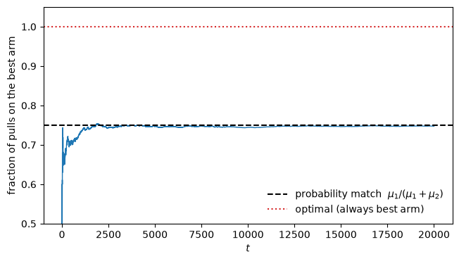
Fig. 88.4 The classifier bandit converges to probability matching#
The fraction of pulls on the better arm converges, but not to one.
It converges to \(\mu_1/(\mu_1 + \mu_2)\), the arm’s share of total expected reward.
for μ in ([1.0, 0.5], [2.0, 1.0], [3.0, 1.0]):
    frac = np.mean(two_armed_bandit(μ)[-5000:] == 0)
    print(f"μ = {μ}: fraction on best arm = {frac:.3f}, "
          f"probability match = {μ[0]/(μ[0]+μ[1]):.3f}  (optimal = 1.0)")
μ = [1.0, 0.5]: fraction on best arm = 0.655, probability match = 0.667  (optimal = 1.0)
μ = [2.0, 1.0]: fraction on best arm = 0.659, probability match = 0.667  (optimal = 1.0)
μ = [3.0, 1.0]: fraction on best arm = 0.750, probability match = 0.750  (optimal = 1.0)
Arthur and Simon proved this: the strength-proportional classifier probability-matches.
It plays the arms in proportion to their expected rewards rather than concentrating on the best one, so it leaves reward on the table forever.
That is not a bug to paper over; it is a lesson about accounting.
A classifier system is only as good as the scheme by which strength is assigned and passed around.
The naive rule here matches probabilities; better rules do better.
And in a sequential problem — where a rule’s payoff comes only much later, through a chain of intermediate decisions — the accounting must do something harder still: reward a rule for merely setting up a profitable future decision.
Holland’s device for this is the bucket brigade: each acting classifier pays part of its strength to the classifier that acted just before it, the one that moved the system into the state where the current rule could act.
Reward paid at the end of a chain seeps backward, rule by rule, until early setup rules that never touch a payoff directly acquire strength for enabling it.
Designing that backward flow is the central craft of building a classifier system, and it is exactly what Money as a Medium of Exchange among Artificially Intelligent Agents must get right to make agents learn to accept money today for the sake of a trade tomorrow.
88.6. Evolutionary programming#
We have surveyed four brains.
The last idea is about what to do with them.
A recurring finding of this whole section is that systems of adaptive agents, however plodding, tend to converge on rational expectations equilibria.
Adaptive Agents in an Overlapping Generations Monetary Economy and Learning, Approximation, and Equilibrium Computation showed least squares learners finding one; Exchange Rate Indeterminacy, Learning, and Experiments showed Newton learners settling on one (of many).
Evolutionary programming turns that tendency into a tool.
If a population of adaptive agents reliably converges to an equilibrium, we can run the population as a method for computing the equilibrium, especially in models too complicated to solve by hand.
Sargent is careful about what is and isn’t going on:
The adaptive agents are ‘teaching’ the economist in the same sense that any numerical algorithm for solving nonlinear equations ‘teaches’ a mathematician. When these agents can ‘teach’ us something, it is because we designed them to do so.
This is the same duality that ran through Learning, Approximation, and Equilibrium Computation: a learning economy is a decentralized equilibrium computation, and an equilibrium computation is a centralized learning algorithm.
The genetic algorithm and the classifier system are simply richer computational engines than recursive least squares, able to search rugged landscapes and to discover the structure of a good rule, not just tune the coefficients of a fixed one.
The showcase is Kiyotaki and Wright [1989]’s search-theoretic model of money, in which the medium of exchange is not assumed but must emerge from how agents choose to trade.
The equilibrium is a set of trading strategies and matching probabilities, and for enriched versions of the model it is hard to characterize analytically.
Marimon et al. [1990] put populations of Holland classifier systems into that environment and watched them converge to an equilibrium, then built a five-good version, with no known analytical solution, and let the classifier systems suggest what the equilibrium looked like.
88.7. Concluding remarks#
The four brains in this catalogue differ in what they take as given.
The perceptron is handed a functional form and asked only for its coefficients, which is why an econometrician recognizes it immediately.
The Hopfield network is handed the patterns themselves and asked only to recall them.
The genetic algorithm is handed nothing but a fitness function and must search a space in which it cannot compute a gradient.
The classifier system is handed a vocabulary in which rules can be written and must discover which rules are worth holding.
Moving down that list, we hand the agent less and ask it to find more, which is precisely the direction the bounded-rationality program pushes us.
Two cautions emerged along the way, and both return in the next lecture.
The genetic algorithm’s individuals do not learn: only the population does, which makes it a model of a society rather than of a mind.
And the bandit showed that a classifier system’s performance is decided by its accounting — by how strength is assigned, bid, and passed along — rather than by the fact of having classifiers at all.
Money as a Medium of Exchange among Artificially Intelligent Agents assembles this machinery into agents who learn, from scratch, to use money, and both cautions bear directly on what those agents turn out to be able to learn.
88.8. Exercises#
Exercise 88.1
The Hopfield network’s recall is descent on the energy \(E(s) = -\tfrac{1}{2}s^\top ws\).
Verify the descent directly.
Take a stored letter, corrupt several pixels, and record the energy at each step of the recall dynamics.
Confirm that energy never increases and that recall halts at (or below) the stored pattern’s energy.
Then corrupt patterns more heavily and classify the failures: does recall land on a different stored letter, or on a spurious state that was never stored?
Compare the energies in each case, and use them to explain why the error happens.
Solution
def recall_with_energy(w, s0, max_iter=30):
    s = s0.copy()
    trace = [energy(w, s)]
    for _ in range(max_iter):
        s_new = np.sign(w @ s)
        s_new[s_new == 0] = 1
        trace.append(energy(w, s_new))
        if np.array_equal(s_new, s):
            break
        s = s_new
    return s, trace

rng = np.random.default_rng(1)
i = letters.index('E')
corrupt = σ[i].copy()
corrupt[rng.choice(25, 5, replace=False)] *= -1
final, trace = recall_with_energy(w_hop, corrupt)

print(f"energy along the recall path: {[round(e, 2) for e in trace]}")
print(f"monotonically non-increasing: {all(np.diff(trace) <= 1e-9)}")
print(f"recovered the intended letter 'E': {np.array_equal(final, σ[i])}")
energy along the recall path: [np.float64(-6.38), np.float64(-12.5), np.float64(-12.5)]
monotonically non-increasing: True
recovered the intended letter 'E': True
The energy falls monotonically along every recall path: the dynamics can only move downhill, which is why the network always halts at a local minimum.
Now corrupt more heavily and sort the outcomes into three kinds: the intended letter, a different stored letter, and a spurious state that is a fixed point but was never taught.
def classify_outcome(final, i):
    if np.array_equal(final, σ[i]):
        return "intended"
    if any(np.array_equal(final, σ[k]) for k in range(len(letters))):
        return "wrong letter"
    return "spurious"

counts = {"intended": 0, "wrong letter": 0, "spurious": 0}
wrong_energy, spurious_energy = [], []
for i in range(len(letters)):
    for seed in range(200):
        r = np.random.default_rng(1000*i + seed)
        corrupt = σ[i].copy()
        corrupt[r.choice(25, 7, replace=False)] *= -1
        final = recall(w_hop, corrupt)
        kind = classify_outcome(final, i)
        counts[kind] += 1
        if kind == "wrong letter":
            wrong_energy.append(energy(w_hop, final))
        elif kind == "spurious":
            spurious_energy.append(energy(w_hop, final))

print(f"7-pixel corruptions ({sum(counts.values())} trials): {counts}")
print(f"stored patterns all have energy {energy(w_hop, σ[0]):.1f}")
print(f"wrong-letter results: energy in [{min(wrong_energy):.1f}, {max(wrong_energy):.1f}]")
print(f"spurious results:     energy in [{min(spurious_energy):.1f}, {max(spurious_energy):.1f}]")
7-pixel corruptions (1000 trials): {'intended': 404, 'wrong letter': 62, 'spurious': 534}
stored patterns all have energy -12.5
wrong-letter results: energy in [-12.5, -12.5]
spurious results:     energy in [-12.5, -10.4]
Both failure modes occur, and at this level of corruption the spurious states are the more common of the two by some margin.
A wrong-letter result sits at exactly the stored energy \(-N/2\): the corruption pushed the starting point clear across a basin boundary, into the domain of attraction of a different stored memory that is just as deep.
Energy descent converges to a minimum but cannot guarantee the nearest one when correlated patterns have interlocking basins.
A spurious result is a local minimum the designer never intended, typically a blend of stored patterns, created as an artifact of the storage rule.
Its energy ranges from shallower than the stored patterns’ all the way down to exactly their depth, so depth alone does not identify a memory as one we asked for.
Some of the deepest spurious states are sign reversals: because \(\operatorname{sgn}(w(-s)) = -\operatorname{sgn}(ws)\), the vector \(-\sigma\) is a fixed point of the same energy whenever \(\sigma\) is, and the network stores each letter’s photographic negative whether we wanted it or not.
Because all of these are genuine local minima, downhill dynamics cannot escape any of them.
Both are why the network is imperfect, and both are why simulated annealing matters: adding declining random shaking lets the system hop out of a shallow spurious basin, or across a basin boundary, before settling, something pure energy descent can never do.
Exercise 88.2
The genetic algorithm’s exploration comes from two operators, crossover and mutation.
The book argues that crossover “lies at the heart of the algorithm,” while mutation alone “is a poor mechanism for injecting diversity.”
Test the claim on Axelrod’s game.
Write a mutation-only variant (each child is a mutated copy of one selected parent, with no crossover) and compare the fitness it reaches against the full algorithm.
The book is careful to say when mutation alone is weak: “when the mutation rate is set to a very low value, mutation alone is a poor mechanism for injecting diversity.”
So run the comparison at a low mutation rate, where crossover has to carry the exploration.
Solution
def evolve_no_crossover(N=60, generations=60, p_mut=0.005, seed=0):
    "Mutation-only variant: each child is a mutated copy of one selected parent."
    rng = np.random.default_rng(seed)
    pop = rng.integers(0, 2, (N, 70))
    best_hist = []
    for _ in range(generations):
        fit = np.array([fitness(pop[i]) for i in range(N)])
        best_hist.append(fit.max())            # recorded exactly as in `evolve`
        weight = fit - fit.min() + 1e-6
        parents = np.searchsorted(np.cumsum(weight), rng.random(N) * weight.sum())
        nxt = pop[parents].copy()
        nxt[rng.random((N, 70)) < p_mut] ^= 1
        pop = nxt
    return best_hist[-1]

rows = []
for seed in range(5):
    panel_rng = np.random.default_rng(seed)
    with_x = evolve(N=60, generations=60, p_mut=0.005, seed=seed)[1][-1]
    panel_rng = np.random.default_rng(seed)
    without_x = evolve_no_crossover(seed=seed)
    rows.append((seed, with_x, without_x))

print(f"{'seed':>4} {'with crossover':>16} {'mutation only':>16}")
for sd, a, b in rows:
    print(f"{sd:>4} {a:>16.3f} {b:>16.3f}")
print(f"{'mean':>4} {np.mean([r[1] for r in rows]):>16.3f} "
      f"{np.mean([r[2] for r in rows]):>16.3f}")
seed   with crossover    mutation only
   0            2.643            2.572
   1            2.540            2.583
   2            2.664            2.547
   3            2.657            2.616
   4            2.669            2.556
mean            2.635            2.575
At a low mutation rate crossover clearly wins: it reaches a higher fitness than the mutation-only variant on almost every seed.
The reason is the one the book gives.
With little mutation, a mutation-only population can only inch forward one rare bit-flip at a time, and quickly loses diversity as selection copies its few best strings.
Crossover instead recombines whole segments that have already proved useful in different strings: a good way of handling one opponent spliced onto a good way of handling another.
It injects large, structured variation while preserving the schemata that fitness has already favored, which is why Holland put it at the center of the algorithm.
Note
The margin narrows, and can even vanish, at higher mutation rates: when mutation is generating plenty of diversity on its own, crossover’s contribution is less pivotal.
Try re-running the comparison at p_mut=0.02 to see the effect shrink.
Whether crossover is decisive depends on the mutation rate and on whether the encoding lines up useful building blocks with contiguous bit segments, which, for this history-indexed strategy table, it only partly does.
Exercise 88.3
The two-armed bandit classifier probability-matches, which is suboptimal: it keeps pulling the worse arm a fixed fraction of the time forever.
A natural fix is to make the auction greedier as the system gains confidence.
Replace the strength-proportional choice rule with a softmax,
where \(\beta\) controls greediness (\(\beta \to \infty\) always picks the stronger arm).
Implement it and show how the long-run fraction on the best arm depends on \(\beta\).
How large must \(\beta\) be to move the classifier from probability matching toward the optimal policy?
Solution
def bandit_softmax(μ, β, σ=0.5, T=20_000, seed=0):
    rng = np.random.default_rng(seed)
    S = np.ones(2)                             # equal strengths, as before
    τ = np.array([1, 1])
    pulls = np.empty(T, int)
    for t in range(T):
        p1 = 1 / (1 + np.exp(-β * (S[0] - S[1])))
        i = 0 if rng.random() < p1 else 1
        reward = μ[i] + σ * rng.standard_normal()
        τ[i] += 1
        S[i] += (reward - S[i]) / τ[i]
        pulls[t] = i
    return np.mean(pulls[-5000:] == 0)

μ = [3.0, 1.0]
print(f"probability match target = {μ[0]/(μ[0]+μ[1]):.3f},  optimal = 1.000\n")
for β in (0.5, 1.0, 2.0, 4.0, 8.0):
    frac = bandit_softmax(μ, β)
    print(f"β = {β:>4}: fraction on best arm = {frac:.3f}")
probability match target = 0.750,  optimal = 1.000

β =  0.5: fraction on best arm = 0.732
β =  1.0: fraction on best arm = 0.888
β =  2.0: fraction on best arm = 0.980
β =  4.0: fraction on best arm = 1.000
β =  8.0: fraction on best arm = 1.000
As \(\beta\) rises the classifier abandons probability matching and concentrates on the better arm, approaching the optimal policy of always pulling it.
The exercise makes concrete why the accounting and auction rules — not just the fact of having classifiers — determine how well a classifier system performs.
The strength-proportional rule of Arthur and Simon is one point on a spectrum; a greedy rule sits at the other end.
Real classifier systems, including the one in Money as a Medium of Exchange among Artificially Intelligent Agents, choose their auction and strength-update rules deliberately, precisely because the choice is what separates a system that merely matches probabilities from one that learns to act well.