84. A Peculiar Definition of Bounded Rationality#
84.1. Overview#
This lecture opens a series based on Sargent [1993] about Bounded Rationality in Macroeconomics, from one point of view in the late 1980s and early 1990s.
Those were years when the Soviet Union ended and formerly Warsaw Pact countries were rearranging their political economies.
For those countries, those were thus truly regime changes in the technical sense of modern dynamic macroeconomics.
Two generations of work on economic dynamics — in game theory, macroeconomics, and general equilibrium theory — had produced theories that embraced the rational expectations assumption, models that were designed to understand settings in which people face recurrent situations they have lived through many times before.
The transitions across regimes underway in Eastern Europe in the early 1990s were not like that.
People there were confronted with unprecedented opportunities, new and ill-defined rules, and a daily struggle to figure out the mechanism that would eventually govern trade and production.
Economists with good models of a market economy had ample equilibrium theories describing how a system behaves once it has fully adjusted to a new and coherent set of rules and expectations.
They knew much less about the dynamics of transitions from a Soviet system to a market economy.
They might hold prejudices and anecdotes about how to manage such a transition, but no empirically confirmed formal theory of it.
Against this background, some economists ventured into what Sims [1980] called the “wilderness” of irrational expectations and bounded rationality.
The aim was partly to build theories of transition dynamics, partly to understand the properties of equilibrium dynamics themselves, and partly to study systems that never settle down.
This series follows Sargent [1993] a little way into that wilderness.
84.1.1. The knowledge that rational expectations imputes#
To see what bounded rationality retreats from, start with rational expectations, which imposes two requirements:
Individual rationality — each artificial agent’s behavior maximizes an objective function subject to perceived constraints.
Mutual consistency — the constraints perceived by everybody in the system agree with one another.
The second requirement is Muth’s rational expectations assumption.
In an economy one person’s decisions are part of another person’s constraints, so consistency requires each person to hold correct beliefs about everyone else’s decisions, decision processes, and beliefs.
Consistency is also what gives rational expectations its power: without some restriction on perceptions, a model in which behavior depends on arbitrary assumptions about subjective beliefs can produce almost any outcome at all.
But look at what that requirement imputes to people once a model is taken to data.
The agents inside a rational expectations model evaluate their Euler equations using equilibrium probability distributions.
Those are the very distributions that the econometrician studying them is still struggling to estimate.
The agents, in other words, have somehow already solved the inference problem that the economist is only part way through.
84.1.2. Sargent’s formulation of bounded rationality#
Sargent’s bounded rationality program keeps individual rationality and retreats from mutual consistency in a particular way that was motivated by his love of time series econometrics.
Sargent’s version of a bounded rationality program is:
I interpret a proposal to build models with ‘boundedly rational’ agents as a call to retreat from the second piece of rational expectations (mutual consistency of perceptions) by expelling rational agents from our model environments and replacing them with ‘artificially intelligent’ agents who behave like econometricians. These ‘econometricians’ theorize, estimate, and adapt in attempting to learn about probability distributions which, under rational expectations, they already know.
The agents are made more like the people who build the models: they gather data, form theories, estimate, and adapt.
Note
After he saw Sargent’s manuscript, Carnegie-Mellon’s Herbert Simon wrote Sargent a letter saying that he objected to Sargent’s formulation and recommended that Sargent not call what he was doing ‘‘bounded rationality’’.
Simon particularly disliked Sargent’s making the agents inside his model act like econometricians, a pretense that Simon found preposterous.
Sargent’s proposal makes work harder for the model builder, not easier.
Withdrawing the assumption of a commonly understood environment means we must put something in its place, and there are many plausible somethings to choose among:
This area is wilderness because the researcher faces so many choices after he decides to forgo the discipline provided by equilibrium theorizing. The commitment to equilibrium theorizing made many choices for him by requiring that people be modelled as optimal decision-makers within a commonly understood environment. When we withdraw the assumption of a commonly understood environment, we have to replace it with something, and there are so many plausible possibilities.
84.1.3. What the program is good for#
The payoffs the book pursues are of three kinds.
Sometimes a collection of adaptive agents learns to behave as if it had rational expectations, which lends the equilibrium a plausibility it lacked as a mere assumption.
Sometimes adaptive agents converge to a particular equilibrium among many, turning learning into a device for selecting among rational expectations equilibria, and, relatedly, into a way of computing equilibria too complicated to solve by hand.
And, more ambitiously, adaptive dynamics hold out the hope of a theory of the transition itself, the out-of-equilibrium adjustment that the Eastern European reformers had to manage blind.
That last promise is the least fulfilled, as the series will acknowledge; the selection and computation payoffs are the surer ones.
This lecture takes up selection, through the sharpest case: models with too many equilibria.
When a rational expectations model has a continuum of equilibria, the physical description of the economy plus the equilibrium concept fail to pin down what happens.
Something else must choose, and a plausible account of how people grope toward equilibrium is a natural candidate for that something.
We build the two monetary examples that the rest of the series returns to repeatedly, both with a continuum of rational expectations equilibria:
a quantity-theory model of money and prices in which the price level is determined only up to an arbitrary bubble term, and
a two-currency version in which the exchange rate is completely unrestricted.
Along the way we set up the machinery — the fixed-point view of equilibrium, the relaxation algorithm, adaptive expectations, and Muth’s inverse optimal-prediction problem — that later lectures use to expel the rational agents and put adaptive ones in their place.
84.1.4. The rest of the series#
Adaptive Agents in an Overlapping Generations Monetary Economy — adaptive households in Samuelson’s overlapping generations monetary model.
Least squares learning selects the low-inflation equilibrium that the rational expectations dynamics reject, and laboratory subjects go the same way.
A government learning a Phillips curve closes the lecture.
Learning, Approximation, and Equilibrium Computation — what an agent must give up when the state is continuous and a separate response for each contingency is out of the question, which brings in approximate equilibria and the resemblance between learning algorithms and equilibrium computation algorithms.
Exchange Rate Indeterminacy, Learning, and Experiments — the two-currency model of this lecture with adaptive agents, where learning pins the exchange rate down only by making it depend on history, while a genetic-algorithm economy instead produces volatility that never dies.
Genetic Algorithms and Classifier Systems — a catalogue of candidate brains, from Holland and the connectionists: perceptrons, associative memories, genetic algorithms, classifier systems.
Money as a Medium of Exchange among Artificially Intelligent Agents — populations of classifier systems that discover, from scratch, which good will serve as money.
1993 Prospects for Bounded Rationality in Macroeconomics — the 1993 ledger of what the program achieved and what it did not, and a postscript on the three decades since.
Let’s start with some imports.
import numpy as np
import pandas as pd
import matplotlib.pyplot as plt
84.2. Rational expectations as a fixed point#
84.2.1. A static market#
Take a competitive industry with a large number \(n\) of identical firms.
Each firm chooses output \(x\) to maximize
where \(c\) is an increasing, convex cost function, and price is determined by a downward-sloping inverse demand curve
in which \(X\) is the output of the average firm.
Each firm is a price-taker and an \(X\)-taker: it takes \(p\) as given and sets marginal cost equal to price, \(p = c'(x)\).
Write the solution as \(x = g(p)\).
Substituting the demand curve gives the best-response map
which sends a conjectured industry average \(X\) to the individual output an optimizing firm would choose against it.
That is the first component of rational expectations, and it is all that individual rationality delivers.
The second component — consistency — requires that what each firm chooses coincides with what it assumed the average firm was choosing:
A static rational expectations equilibrium is a fixed point of the best-response map.
For a concrete example, take a quadratic cost function \(c(x) = \tfrac{\gamma}{2} x^2\) and a linear inverse demand curve \(p = a - b n X\).
Then \(p = c'(x) = \gamma x\) gives \(x = p / \gamma\), so
a, b, n, γ = 10.0, 0.3, 5, 1.0

def h(X):
    "Best response of an individual firm to an industry average X."
    return (a - b * n * X) / γ

X_star = a / (γ + b * n)
print(f"X*     = {X_star}")
print(f"h(X*)  = {h(X_star)}")
print(f"h'(X)  = {-b * n / γ}")
X*     = 4.0
h(X*)  = 4.0
h'(X)  = -1.5
84.2.2. Computing the fixed point#
Now suppose we want to find \(X^*\) without solving for it in closed form.
A natural starting point is the relaxation algorithm: carry an estimate \(X^*_k\) of the equilibrium, compute the best response to it, and move part of the way toward that best response,
where \(\lambda \in (0, 1]\) is a relaxation parameter.
With \(\lambda = 1\) this is simple iteration on \(h\), the classic cobweb.
def relax(λ, X0=1.0, n_iter=12):
    "Iterate the relaxation algorithm, returning the whole path."
    path = np.empty(n_iter + 1)
    path[0] = X0
    for k in range(n_iter):
        path[k + 1] = path[k] + λ * (h(path[k]) - path[k])
    return path


fig, axes = plt.subplots(1, 2, figsize=(11, 4))

axes[0].plot(relax(1.0), 'o-', ms=4, lw=1, color='C0',
             label=r"$\lambda = 1.0$ (cobweb)")
axes[0].set_title("undamped")
axes[0].set_ylabel("$X^*_k$")

for i, λ in enumerate((0.8, 0.5, 0.3)):
    axes[1].plot(relax(λ), 'o-', ms=4, lw=1, color=f'C{i+1}',
                 label=fr"$\lambda = {λ}$")
axes[1].set_title("damped")
axes[1].set_ylim(-1, 9)

for ax in axes:
    ax.axhline(X_star, color='k', lw=0.8, ls='--', label="$X^*$")
    ax.set_xlabel("$k$")
    ax.legend(frameon=False, fontsize=9)
plt.tight_layout()
plt.show()
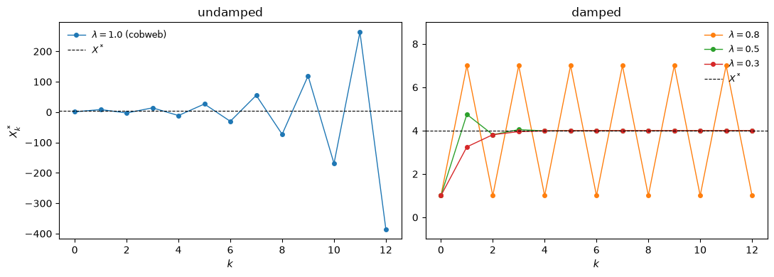
Fig. 84.1 Relaxation algorithm paths, undamped and damped#
The naive cobweb \(\lambda = 1\) diverges, oscillating ever further away from the equilibrium it is trying to find; note the scale on the left panel.
Since \(h\) is affine, iteration (84.3) has multiplier \(1 + \lambda(h' - 1)\), so it converges if and only if
λ_max = 2 / (1 + b * n / γ)
print(f"converges iff λ < {λ_max}")
print(f"λ = 1.0 : multiplier = {1 + 1.0 * (-b*n/γ - 1):+.2f}   (diverges)")
print(f"λ = 0.8 : multiplier = {1 + 0.8 * (-b*n/γ - 1):+.2f}   (period-2 cycle)")
print(f"λ = 0.5 : multiplier = {1 + 0.5 * (-b*n/γ - 1):+.2f}   (converges)")
converges iff λ < 0.8
λ = 1.0 : multiplier = -1.50   (diverges)
λ = 0.8 : multiplier = -1.00   (period-2 cycle)
λ = 0.5 : multiplier = -0.25   (converges)
At \(\lambda = 0.8\) the multiplier is exactly \(-1\): the scheme maps \(X \mapsto 8 - X\) and so bounces forever between \(1\) and \(7\) without either converging or diverging, which is the undamped zigzag in the right panel.
Damping the adjustment enough makes the algorithm find the equilibrium; not damping it enough makes the algorithm chase its own tail.
Hold on to that observation.
A recurring theme of this series is that how you adapt determines where, and whether, you end up.
84.2.3. Adaptive expectations#
Equation (84.3) was introduced as an algorithm running in iteration count \(k\).
Reinterpret \(k\) as calendar time \(t\), read \(X^*_t\) as the value people expect, and \(X_t = h(X^*_{t-1})\) as what actually happens, and it becomes a theory of expectation formation:
This is the adaptive expectations scheme that Cagan [Cagan, 1956] used to study hyperinflations and that Friedman used to study consumption.
Expectations are a geometrically declining distributed lag of past observations, with a single free parameter \(\lambda\) describing beliefs.
Cagan and Friedman took \(\lambda\) as a free parameter and left open the question of why anyone would form expectations this way.
84.2.4. Muth’s inverse problem#
Muth [1960] set out to eliminate \(\lambda\) as a free parameter by turning the question around.
Instead of asking what forecasts a given environment implies, he asked: for what environment would exponential smoothing be the optimal forecast?
His answer is that (84.4) is the least-squares forecast of \(X_{t+k}\) at every horizon \(k\) if and only if \(X_t\) follows
with \(\{\epsilon_t\}\) a martingale difference sequence, and the smoothing weight tied to the moving-average coefficient by
Note
Sargent writes both the smoothing weight in (84.4) and the moving-average coefficient in (84.5) as \(\lambda\).
We use \(\theta\) for the second to keep the relationship \(\lambda = 1 - \theta\) visible.
Two other symbols work double shifts in this lecture, both following the book.
In the money model below, \(\lambda\) is no longer a gain but the gross growth rate \(w_1/w_2\) of the bubble term, and \(\gamma\) is no longer the curvature of a cost function but the coefficient linking the price level to the money supply.
The code distinguishes them as λ_m and γ_m.
The forecasting rule inherits its one parameter from the stochastic process being forecast.
Let’s confirm this numerically: simulate (84.5), run exponential smoothing at a range of weights, and see which weight forecasts best.
def smoothing_mse(x, λ):
    "One-step-ahead forecast MSE of exponential smoothing with weight λ."
    f = np.empty_like(x)
    f[0] = x[0]
    for i in range(1, len(x)):
        f[i] = λ * x[i] + (1 - λ) * f[i - 1]
    return np.mean((x[1:] - f[:-1]) ** 2)


rng = np.random.default_rng(0)
T = 200_000
ε = rng.standard_normal(T + 1)           # one shock path, shared across all λ
grid = np.linspace(0.02, 0.98, 97)

fig, ax = plt.subplots(figsize=(7, 4))
for θ in (0.2, 0.5, 0.8):
    X = np.cumsum(ε[1:] - θ * ε[:-1])    # Muth's process
    mse = np.array([smoothing_mse(X, λ) for λ in grid])
    line, = ax.plot(grid, mse, lw=1.2, label=fr"$\theta = {θ}$")
    ax.axvline(1 - θ, color=line.get_color(), lw=0.8, ls='--')
    print(f"θ = {θ}:  best λ = {grid[mse.argmin()]:.2f},  1 - θ = {1 - θ:.2f},"
          f"  min MSE = {mse.min():.4f}")
ax.set_xlabel(r"smoothing weight $\lambda$")
ax.set_ylabel("forecast MSE")
ax.set_ylim(0.9, 3)
ax.legend(frameon=False)
plt.show()
θ = 0.2:  best λ = 0.80,  1 - θ = 0.80,  min MSE = 1.0024
θ = 0.5:  best λ = 0.50,  1 - θ = 0.50,  min MSE = 1.0024
θ = 0.8:  best λ = 0.20,  1 - θ = 0.20,  min MSE = 1.0024
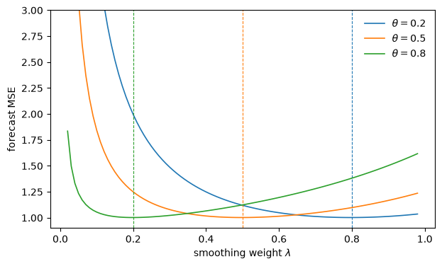
Fig. 84.2 Forecast MSE of exponential smoothing#
Each curve bottoms out exactly at its dashed line \(\lambda = 1 - \theta\), and the minimized mean squared error is \(\mathbb{V}[\epsilon_t] = 1\) up to simulation noise — exponential smoothing at that weight is the conditional expectation, and nothing can beat it.
Muth’s exercise was the first application of the rational expectations idea in the form that became standard: find the restrictions that link a forecasting scheme to the environment in which it is used.
It also pushed later researchers to treat the forecasting scheme itself as the object in terms of which equilibrium is defined.
84.2.5. The dynamic analogue#
That is exactly what happens when we move from static to dynamic models.
Let each agent choose a sequence rather than a single action, taking as given a perceived law of motion for the aggregate state,
where \(\{u_t\}\) is IID
Solving the agent’s dynamic program yields an individual decision rule \(x_t = h(x_{t-1}, X_{t-1}, u_t)\).
Imposing that the representative agent is representative, \(x_t = X_t\), delivers the actual law of motion
and hence a map from perceived to actual laws of motion,
A dynamic rational expectations equilibrium is a fixed point \(H = T(H)\), the same idea as (84.2), but the fixed point now lives in a space of functions rather than a space of numbers.
The relaxation algorithm carries over unchanged,
except that it now revises entire expectations-generating functions in response to the gap between what they predicted and what happened.
Every learning model in this series is some version of (84.7) with the gain \(\lambda\) made to decline over time and the revision driven by data rather than by an exact evaluation of \(T\).
See also
Rational Expectations Equilibrium develops the \(T\) map in detail for a Lucas–Prescott industry model and computes its fixed point.
Least Squares Learning in Self-Referential Models studies what happens when agents estimate the perceived law of motion by least squares while living inside the system their estimates help determine.
84.3. Money and prices#
We now build the first of the two models that motivate everything that follows.
A representative money-holder chooses nominal balances \(m_t\) to carry from \(t\) to \(t+1\) to maximize
where \(p_t\) is the current price level and \(p^*_{t+1}\) is the price level expected next period.
The first term is consumption today, reduced by the real resources \(m_t / p_t\) given up to acquire currency; the second is consumption tomorrow, augmented by the goods \(m_t / p^*_{t+1}\) that the currency is expected to command.
Differentiating (84.8) with respect to \(m_t\) and rearranging gives the demand for money
Real balances fall when currency is expected to lose value faster.
This is a version of the demand function Cagan [Cagan, 1956] used to study hyperinflations, and it also arises in Samuelson’s [Samuelson, 1958] overlapping generations model.
To close the model we need a theory of \(p^*_{t+1}\).
Suppose the money supply grows at a constant rate,
and that the household believes the price level is related to the money supply by
for constants \((\gamma, \lambda, c)\) that summarize its beliefs, all positive so that the price level stays positive.
Knowing \(\mu\), the household forecasts \(p^*_{t+1} = \gamma \mu M_t + \lambda^{t+1} c\).
Substituting the forecast and (84.11) into (84.9) gives money demand as a function of the current money supply,
Notice a feature common to models in which expectations matter: the demand for money depends on its supply, because today’s demand depends on tomorrow’s expected price level, which is believed to depend on tomorrow’s money supply.
84.3.1. Equilibrium#
Setting demand equal to supply, \(m_t = M_t\), turns (84.12) into a functional equation,
which must hold at every date.
Matching the two terms gives
so the equilibrium price level is
The parameters \(\gamma\) and \(\lambda\) are pinned down.
The constant \(c\) is not.
Every \(c \geq 0\) is a rational expectations equilibrium, and expectations formed from (84.11) are always exactly right in each of them.
Let’s verify that the residual really does vanish for any \(c\) we care to try.
w1, w2, μ, M0 = 2.0, 1.0, 1.5, 1.0
γ_m, λ_m = 1 / (w1 - μ * w2), w1 / w2

t = np.arange(12)
M = M0 * μ ** t

def price_path(c):
    "Equilibrium price level for bubble constant c."
    return γ_m * M + λ_m ** t * c

for c in (0.0, 0.5, 3.0, 25.0):
    p = price_path(c)
    p_star = γ_m * μ * M + λ_m ** (t + 1) * c     # forecast of next period's price
    m = w1 * p - w2 * p_star                      # money demand
    print(f"c = {c:5}:  max |demand - supply| = {np.max(np.abs(m - M)):.2e}")
c =   0.0:  max |demand - supply| = 0.00e+00
c =   0.5:  max |demand - supply| = 0.00e+00
c =   3.0:  max |demand - supply| = 0.00e+00
c =  25.0:  max |demand - supply| = 0.00e+00
Money demand equals money supply exactly, at every date, for every \(c\).
84.3.2. The bubble#
Since \(w_1 > w_2\), the second term in (84.14) grows at the gross rate \(\lambda = w_1 / w_2 > 1\).
In the equilibrium with \(c = 0\) the price level is proportional to the money supply: the quantity theory in its textbook form.
In every other equilibrium the price level carries a component that has nothing to do with the money supply and grows exponentially: a purely speculative bubble.
fig, axes = plt.subplots(1, 2, figsize=(11, 4))

for c in (0.0, 0.5, 3.0):
    lab = f"$c = {c}$" + (" (quantity theory)" if c == 0 else "")
    axes[0].plot(t, price_path(c), 'o-', ms=3, lw=1, label=lab)
    axes[1].plot(t, M / price_path(c), 'o-', ms=3, lw=1, label=lab)

axes[0].set_yscale('log')
axes[0].set_ylabel("$p_t$  (log scale)")
axes[1].set_ylabel("real balances  $M_t / p_t$")
axes[1].axhline(w1 - μ * w2, color='k', lw=0.8, ls='--')
axes[1].set_ylim(0, 0.6)
for ax in axes:
    ax.set_xlabel("$t$")
    ax.legend(frameon=False, fontsize=9)
plt.tight_layout()
plt.show()
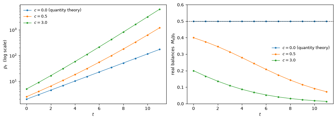
Fig. 84.3 Price levels and real balances under bubbles#
The left panel shows the price level diverging further and further from the quantity-theory path as \(c\) rises.
The right panel shows what that does to the real value of the money stock: with \(c = 0\) real balances are constant at \(w_1 - \mu w_2\), while with \(c > 0\) the bubble drives them steadily toward zero.
Along a bubble path the gross inflation rate climbs toward \(w_1 / w_2\), which from (84.9) is precisely the rate at which the demand for real balances vanishes.
The economy demonetizes itself, purely because everyone expects it to.
infl = pd.DataFrame(
    {f"c = {c}": price_path(c)[1:] / price_path(c)[:-1] for c in (0.0, 0.5, 3.0)},
    index=pd.Index(t[1:], name="t"),
).round(3)
infl
| c = 0.0 | c = 0.5 | c = 3.0 | |
|---|---|---|---|
| t | |||
| 1 | 1.5 | 1.600 | 1.800 |
| 2 | 1.5 | 1.625 | 1.833 |
| 3 | 1.5 | 1.654 | 1.864 |
| 4 | 1.5 | 1.686 | 1.890 |
| 5 | 1.5 | 1.721 | 1.913 |
| 6 | 1.5 | 1.757 | 1.932 |
| 7 | 1.5 | 1.792 | 1.947 |
| 8 | 1.5 | 1.826 | 1.959 |
| 9 | 1.5 | 1.857 | 1.969 |
| 10 | 1.5 | 1.885 | 1.976 |
| 11 | 1.5 | 1.908 | 1.982 |
There is nothing in the model — no preference, no technology, no policy — that says which \(c\) we are in.
Rational expectations, as the paper puts it, “is not a sufficiently restrictive principle to determine outcomes.”
84.4. Two currencies#
The indeterminacy gets worse when we allow more than one currency.
Following Kareken and Wallace [1981], keep (84.9) as the demand for currency in total, and suppose there are two fiat currencies in supplies \(M_{1t}\) and \(M_{2t}\) that are perfect substitutes as long as their rates of return are equal:
This indifference about which currency to hold is what makes the exchange rate indeterminate.
Let people believe the price levels are given by
where \(e\) is a constant exchange rate.
Requiring that the demand for currency, valued in units of currency 1, equal the total supply \(M_{1t} + e M_{2t}\) gives
These equations are remarkable for what they leave out.
The exchange rate \(e\) is entirely unrestricted — if the equations have a solution for one \(e\), they have a solution for every other — and the formulas for \(\gamma_1\) and \(\gamma_2\) do not involve \(e\) at all.
Take the simplest case: two currencies in fixed supply, \(\mu_1 = \mu_2 = 1\), and set \(c = 0\).
Then \(\gamma_1 = \gamma_2 = (w_1 - w_2)^{-1}\) and the price levels are constant.
w1, w2 = 2.0, 1.0
H1, H2 = 100.0, 120.0                 # fixed supplies of the two currencies
γ_e = 1 / (w1 - w2)

def two_currency(e):
    "Price levels and the real allocation at exchange rate e."
    p1 = γ_e * (H1 + e * H2)
    p2 = p1 / e
    supply = H1 + e * H2              # total currency, in units of currency 1
    demand = (w1 - w2) * p1           # money demand, with p* = p since prices are constant
    return p1, p2, supply / p1, demand - supply

pd.DataFrame(
    [two_currency(e) for e in (0.25, 0.5, 1.0, 2.0, 4.0)],
    index=pd.Index([0.25, 0.5, 1.0, 2.0, 4.0], name="e"),
    columns=["$p_1$", "$p_2$", "real balances", "excess demand"],
).round(4)
| $p_1$ | $p_2$ | real balances | excess demand | |
|---|---|---|---|---|
| e | ||||
| 0.25 | 130.0 | 520.0 | 1.0 | 0.0 |
| 0.50 | 160.0 | 320.0 | 1.0 | 0.0 |
| 1.00 | 220.0 | 220.0 | 1.0 | 0.0 |
| 2.00 | 340.0 | 170.0 | 1.0 | 0.0 |
| 4.00 | 580.0 | 145.0 | 1.0 | 0.0 |
Every row is an equilibrium.
The nominal price levels move around a great deal as \(e\) varies.
Since \(e\) is the value of a unit of currency 2 in units of currency 1, a larger \(e\) means currency 2 is worth more, which raises \(p_1\) and lowers \(p_2\).
But the last two columns tell the real story: total real balances are \(w_1 - w_2 = 1\) regardless of \(e\), and markets clear exactly.
The real allocation is identical in every one of these equilibria. The model determines what people consume and how much purchasing power the currency stock commands; it says nothing whatever about the rate at which the two monies exchange.
This is a sharp version of a problem that has haunted international monetary theory, and it is not a knife-edge case: it is a continuum.
84.5. Where this leaves us#
We now have two models in which rational expectations is silent about something we would very much like to predict.
There are three ways to respond.
The first is to add restrictions to the environment until the equilibrium becomes unique.
The second is to declare the indeterminacy a genuine feature of the world.
The third — the one this series pursues — is to ask what happens when we replace the rational agents with adaptive ones and watch where the system goes.
This is a substantive change, not a technicality.
An adaptive agent is not endowed with the equilibrium; it has beliefs, a rule for revising them, and initial conditions.
Those extra objects are exactly what the rational expectations equilibrium conditions failed to pin down, so a system of adaptive agents can select an outcome where rational expectations could not.
The rest of this series takes that idea seriously, and the results are mixed in an instructive way.
In the overlapping generations monetary economy, least squares learning selects the opposite equilibrium from the one the rational expectations dynamics converge to, and human experimental subjects side with the adaptive model.
In the two-currency model above, adaptive agents do pin the exchange rate down, but only by making it depend on initial conditions.
The rest points of the learning algorithm reproduce the indeterminacy exactly, and what selects an outcome is the dead hand of history.
In a Kiyotaki–Wright search economy, adaptive agents learn to use a medium of exchange and select the fundamental equilibrium over the speculative one, even at parameters where theory says the speculative equilibrium is the only one.
In each case the algorithm supplies what the equilibrium concept did not.
Whether that is a discovery about economies or an artifact of the algorithm is the question the series keeps returning to, and 1993 Prospects for Bounded Rationality in Macroeconomics renders a verdict.
84.6. Exercises#
Exercise 84.1
The relaxation algorithm (84.3) converges for the static market if and only if \(\lambda < 2 / (1 + bn/\gamma)\).
The ratio \(bn/\gamma\) measures the slope of demand relative to the curvature of costs, so a market with steep demand and near-linear costs is one in which the naive cobweb (\(\lambda = 1\)) is badly behaved.
Verify the stability boundary numerically: for a grid of values of \(bn/\gamma\), find the largest \(\lambda\) (on a fine grid) for which the algorithm converges, and compare with the analytical prediction.
Solution
def converges(slope, λ, n_iter=400, tol=1e-8):
    """Does the relaxation algorithm converge when h'(X) = -slope?"""
    a_, X = 10.0, 1.0
    for _ in range(n_iter):
        X_new = X + λ * ((a_ - slope * X) - X)
        if not np.isfinite(X_new) or abs(X_new) > 1e12:
            return False
        X, X_prev = X_new, X
    return abs(X - X_prev) < tol


λ_grid = np.linspace(0.01, 1.5, 300)
rows = []
for slope in (0.5, 1.0, 1.5, 2.0, 4.0):
    ok = [λ for λ in λ_grid if converges(slope, λ)]
    rows.append((slope, max(ok) if ok else np.nan, 2 / (1 + slope)))

pd.DataFrame(rows, columns=["$bn/\\gamma$", "largest $\\lambda$ found",
                            "$2/(1 + bn/\\gamma)$"]).round(3)
| $bn/\gamma$ | largest $\lambda$ found | $2/(1 + bn/\gamma)$ | |
|---|---|---|---|
| 0 | 0.5 | 1.296 | 1.333 |
| 1 | 1.0 | 0.972 | 1.000 |
| 2 | 1.5 | 0.777 | 0.800 |
| 3 | 2.0 | 0.648 | 0.667 |
| 4 | 4.0 | 0.389 | 0.400 |
The numerical boundary sits consistently a little below the analytical one, and that gap is not grid spacing; it is a real feature of the test.
As \(\lambda\) approaches the boundary the multiplier approaches \(-1\), so convergence becomes arbitrarily slow, and a test with a fixed iteration count and tolerance declares failure just before the true boundary.
The size of the gap is predictable: with 400 iterations and a tolerance of \(10^{-8}\), the test passes only while \(|1 - \lambda(1 + bn/\gamma)|^{400} \lesssim 10^{-8}\), i.e. while the multiplier is below about \(\exp(-18.4/400) = 0.955\) in absolute value.
predicted = [(1 + 0.955) / (1 + s_) for s_ in (0.5, 1.0, 1.5, 2.0, 4.0)]
pd.DataFrame({"$bn/\\gamma$": [0.5, 1.0, 1.5, 2.0, 4.0],
              "found": [r[1] for r in rows],
              "predicted by the tolerance": predicted,
              "true boundary": [r[2] for r in rows]}).round(3)
| $bn/\gamma$ | found | predicted by the tolerance | true boundary | |
|---|---|---|---|---|
| 0 | 0.5 | 1.296 | 1.303 | 1.333 |
| 1 | 1.0 | 0.972 | 0.978 | 1.000 |
| 2 | 1.5 | 0.777 | 0.782 | 0.800 |
| 3 | 2.0 | 0.648 | 0.652 | 0.667 |
| 4 | 4.0 | 0.389 | 0.391 | 0.400 |
Note the first row: when \(bn/\gamma < 1\) the boundary exceeds one, so the naive cobweb converges on its own and no damping is needed.
Damping is what buys convergence in the steep markets, and the steeper the market the more damping is required.
Exercise 84.2
The equilibrium (84.13) was derived without checking that it makes economic sense.
Show that a monetary equilibrium requires \(\mu < w_1 / w_2\), by finding what goes wrong with the demand for real balances when money grows faster than that.
Solution
Along the \(c = 0\) equilibrium, real balances are constant at \(M_t / p_t = \gamma^{-1} = w_1 - \mu w_2\).
This is positive only when \(\mu < w_1 / w_2\).
If money grows faster, (84.13) still “solves” the functional equation, but it asks the household to hold a negative quantity of currency.
w1, w2 = 2.0, 1.0
μ_grid = np.array([0.5, 1.0, 1.5, 1.9, 2.0, 2.5])

with np.errstate(divide='ignore'):        # γ is infinite exactly at μ = w1/w2
    table = pd.DataFrame({
        "$\\mu$": μ_grid,
        "$\\gamma = (w_1 - \\mu w_2)^{-1}$": 1 / (w1 - μ_grid * w2),
        "real balances $w_1 - \\mu w_2$": w1 - μ_grid * w2,
        "monetary equilibrium?": np.where(μ_grid < w1 / w2, "yes", "no"),
    }).round(3)
table
| $\mu$ | $\gamma = (w_1 - \mu w_2)^{-1}$ | real balances $w_1 - \mu w_2$ | monetary equilibrium? | |
|---|---|---|---|---|
| 0 | 0.5 | 0.667 | 1.5 | yes |
| 1 | 1.0 | 1.000 | 1.0 | yes |
| 2 | 1.5 | 2.000 | 0.5 | yes |
| 3 | 1.9 | 10.000 | 0.1 | yes |
| 4 | 2.0 | inf | 0.0 | no |
| 5 | 2.5 | -2.000 | -0.5 | no |
At \(\mu = w_1 / w_2 = 2\) the demand for real balances hits zero and \(\gamma\) blows up; beyond it, both are negative.
The intuition runs through (84.9): the household holds currency only if the expected loss of purchasing power, \(p^*_{t+1} / p_t\), is smaller than \(w_1 / w_2\).
Money growing at rate \(\mu\) produces inflation at rate \(\mu\), so \(\mu \geq w_1 / w_2\) drives the demand for money to zero, the same boundary that the bubble equilibria approach asymptotically from below.
Exercise 84.3
In the two-currency example we set \(\mu_1 = \mu_2 = 1\) and found that the real allocation was the same at every exchange rate.
That is special.
Repeat the calculation with \(\mu_1 \neq \mu_2\) — say \(\mu_1 = 1.0\) and \(\mu_2 = 1.3\), with \(w_1 = 2\), \(w_2 = 1\), \(M_{1,0} = M_{2,0} = 100\), and \(c = 0\) — and compute total real balances at several exchange rates over the first several periods.
Does the choice of \(e\) still leave the real allocation untouched?
Solution
w1, w2 = 2.0, 1.0
μ1, μ2 = 1.0, 1.3
γ1, γ2 = 1 / (w1 - μ1 * w2), 1 / (w1 - μ2 * w2)
t = np.arange(10)
M1, M2 = 100.0 * μ1 ** t, 100.0 * μ2 ** t

def real_balances(e):
    p1 = γ1 * M1 + γ2 * e * M2
    return (M1 + e * M2) / p1

pd.DataFrame({f"e = {e}": real_balances(e) for e in (0.25, 1.0, 4.0)},
             index=pd.Index(t, name="t")).round(4)
| e = 0.25 | e = 1.0 | e = 4.0 | |
|---|---|---|---|
| t | |||
| 0 | 0.9211 | 0.8235 | 0.7447 |
| 1 | 0.9049 | 0.8050 | 0.7356 |
| 2 | 0.8871 | 0.7879 | 0.7282 |
| 3 | 0.8681 | 0.7725 | 0.7221 |
| 4 | 0.8485 | 0.7591 | 0.7173 |
| 5 | 0.8290 | 0.7476 | 0.7135 |
| 6 | 0.8101 | 0.7380 | 0.7105 |
| 7 | 0.7926 | 0.7301 | 0.7081 |
| 8 | 0.7767 | 0.7237 | 0.7063 |
| 9 | 0.7627 | 0.7186 | 0.7049 |
fig, ax = plt.subplots(figsize=(7, 4))
for e in (0.25, 1.0, 4.0):
    ax.plot(t, real_balances(e), 'o-', ms=3, lw=1, label=f"$e = {e}$")
ax.axhline(1 / γ1, color='k', lw=0.8, ls='--', label=r"$1/\gamma_1$")
ax.axhline(1 / γ2, color='gray', lw=0.8, ls=':', label=r"$1/\gamma_2$")
ax.set_xlabel("$t$")
ax.set_ylabel("total real balances")
ax.legend(frameon=False)
plt.show()
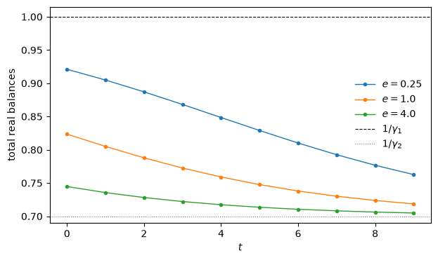
No. With unequal money growth rates the exchange rate affects the real allocation, and the allocation is no longer even constant over time.
The reason is that \(\gamma_1 \neq \gamma_2\): the two currencies are valued differently because they are expected to be diluted at different rates, so the composition of the currency stock matters, and \(e\) is what fixes that composition.
Since currency 2 grows faster, it comes to dominate the stock whatever \(e\) we choose, and real balances converge to \(1/\gamma_2\) from wherever \(e\) starts them.
So the pure nominal indeterminacy of the fixed-supply case is a knife-edge, but the indeterminacy of \(e\) itself is not: every \(e\) in the table is still an equilibrium.