85. Adaptive Agents in an Overlapping Generations Monetary Economy#
85.1. Overview#
A Peculiar Definition of Bounded Rationality presented some models of monetary economies with multiple rational expectations equilibria.
This lecture takes one of them — Samuelson’s overlapping generations model of fiat money, used by Bryant, Wallace and others to study inflationary finance — and replaces Samuelson’s agents who forecast according to the equilibrium law of motion for the price level with ‘‘adaptive’’ ones who do not.
We do this twice, for two different purposes.
Part 1 puts a stochastic government deficit into the model and asks whether successive generations, groping their way by trial and error, can somehow as a society converge to a rational expectations equilibrium.
They can.
Each generation observes what happened to its predecessors and adjusts their saving decision in a utility-improving direction, using a Robbins–Monro recursion.
Given enough time the economy converges to the stationary equilibrium we compute independently.
This exercise also shows how sensitive learning is to the complexity of what must be learned: a deficit state that occurs rarely is learned about slowly, because the observations arrive slowly.
Part 2 removes the randomness and turns to a sharper question.
With a constant deficit the model has two stationary equilibria, one with low inflation and one with high inflation.
The low-inflation equilibrium Pareto-dominates the other.
Under the rational expectations dynamics, the low-inflation equilibrium is unstable and the high-inflation one is stable: theory pushes the economy toward the bad outcome.
Under least squares learning, the stability is reversed.
And when Marimon and Sunder [1993] ran the economy as a laboratory experiment with paid human subjects, the subjects behaved like the adaptive model, not like the rational expectations model.
That is the strongest evidence in Sargent [1993] that adaptive dynamics are doing real work as a selection device, tempered by a counterexample, due to Benjamin Bental, warning against concluding that adaptation reliably selects the good equilibrium.
We then close with a third application, in which the adaptive agent is a government learning a Phillips curve.
Now least squares learning selects the bad, high-inflation equilibrium, but a government that doubts its own model can escape toward the good one, a phenomenon that seeded Sargent’s later work on The Conquest of American Inflation.
Let’s start with some imports.
import numpy as np
import pandas as pd
import quantecon as qe
import matplotlib.pyplot as plt
from scipy.optimize import fsolve
85.2. The environment#
The economy consists of overlapping generations of two-period-lived agents.
At each date \(t \geq 1\), \(N\) identical agents are born, endowed with \(w_1\) units of a single consumption good when young and \(w_2\) units when old.
A young agent’s preferences over lifetime consumption \((c_1, c_2)\) are ordered by the expected value of \(u(c_1) + u(c_2)\).
Throughout we use logarithmic utility, \(u(c) = \ln c\).
A government prints currency to finance expenditures \(G_t\), subject to the budget constraint
where \(H_t\) is the stock of currency carried by the young at \(t\) into \(t+1\), and \(p_t\) is the price level.
Currency is the only store of value, so a young agent’s saving \(s_t\) is entirely in the form of real balances, and market clearing requires
Write \(R_t = p_t / p_{t+1}\) for the gross rate of return on currency between \(t\) and \(t+1\).
Combining (85.1) and (85.2) gives a relation we will use constantly: the return on currency is determined entirely by saving behavior and the deficit,
Currency holds its value only if the next generation is willing to absorb the outstanding stock plus the new issue.
Note
(85.3) is worth pausing on, because it is what makes this a self-referential system, the property studied at length in Least Squares Learning in Self-Referential Models.
The return that today’s young earn on their saving depends on how much tomorrow’s young choose to save, which in turn depends on what tomorrow’s young expect to earn.
Nobody’s beliefs are about an exogenous process.
85.3. Part 1: a stochastic deficit#
Now let government expenditures follow a Markov chain,
over a finite list of levels \(G = [\bar G_1, \ldots, \bar G_n]\).
85.3.1. Stationary rational expectations equilibrium#
In a stationary equilibrium, saving depends on the current deficit state, so it is described by an \(n \times 1\) vector \(s = [s_1, \ldots, s_n]\), and the return on currency by an \(n \times n\) matrix \(R(i,j)\).
A young agent who observes \(G_t = \bar G_i\) chooses \(s_i\) to maximize
with first-order condition
Substituting (85.3) — which in the stationary equilibrium reads \(R(i,j) = (s_j N - \bar G_j)/(s_i N)\) — turns (85.4) into a system of \(n\) nonlinear equations in the saving rates alone:
A stationary equilibrium exists if and only if (85.5) has a solution with \(s_i \in (0, w_1)\) for every \(i\).
w1, w2, N = 20.0, 10.0, 1.0

def u_prime(c):
    return 1 / c                       # log utility

def equilibrium_residual(s, G, P):
    "Left minus right side of the equilibrium condition, one entry per deficit state."
    n = len(s)
    out = np.empty(n)
    for i in range(n):
        rhs = sum(u_prime(w2 + (s[j]*N - G[j])/N)
                  * (s[j]*N - G[j])/(s[i]*N)
                  * P[i, j] for j in range(n))
        out[i] = u_prime(w1 - s[i]) - rhs
    return out

def stationary_equilibrium(G, P, guess=4.0):
    s = fsolve(equilibrium_residual, np.full(len(G), guess), args=(G, P))
    R = np.array([[(s[j]*N - G[j])/(s[i]*N) for j in range(len(s))]
                  for i in range(len(s))])
    return s, R
Following Sargent [1993], we study two economies that differ only in the process for government expenditures, with \(w_1 = 20\), \(w_2 = 10\) and \(N = 1\), so that \(\bar G\) is measured per young person.
In the first, the deficit is always zero and the chain is a fair coin.
G1, P1 = np.array([0.0, 0.0]), np.full((2, 2), 0.5)
s1, R1 = stationary_equilibrium(G1, P1)
print(f"saving rates      {np.round(s1, 4)}")
print(f"returns\n{np.round(R1, 4)}")
saving rates      [5. 5.]
returns
[[1. 1.]
 [1. 1.]]
With no deficit to finance, currency simply holds its value: agents save \(5\) in either state and \(R \equiv 1\).
In the second economy the deficit is \(0.8\) in state 1 and zero in state 2, and the chain is persistent.
G2 = np.array([0.8, 0.0])
P2 = np.array([[0.75, 0.25],
               [0.50, 0.50]])
s2, R2 = stationary_equilibrium(G2, P2)
print(f"saving rates      {np.round(s2, 4)}      (Sargent reports 4.211, 4.364)")
print(f"returns\n{np.round(R2, 4)}")
print("Sargent reports  [[0.81, 1.0362], [0.7817, 1.00]]")
saving rates      [4.2111 4.3637]      (Sargent reports 4.211, 4.364)
returns
[[0.81   1.0362]
 [0.7817 1.    ]]
Sargent reports  [[0.81, 1.0362], [0.7817, 1.00]]
Both match the values reported in the text.
Notice the pattern in \(R\): the return on currency is poor whenever the government is about to run a deficit (the first column), because new issue dilutes the outstanding stock.
85.3.2. Learning by successive generations#
Now withdraw the equilibrium from the agents.
They are still assumed to know their own utility function and to remember the experience of earlier agents like themselves, but they are not told the distribution of returns, which is exactly the object that (85.4) requires.
Instead, each generation adjusts its predecessors’ saving decision in the direction that realized experience suggests would have been better.
The realized lifetime utility of an agent who saved \(s\) and earned \(R\) is
with derivatives
The connection to equilibrium is that in a rational expectations equilibrium \(V'(s_i) = E_t U'(s_i)\) and \(V''(s_i) = E_t U''(s_i)\), where \(E_t\) conditions on \(G_t = \bar G_i\).
So an agent who could compute \(E_t U'\) would just set it to zero and be done.
Our agents cannot, and must estimate it from experience instead.
They use a Robbins–Monro algorithm, applied state by state.
Let \(\tau_i\) count the number of times the deficit state \(\bar G_i\) has been visited so far, and let \(\gamma_\tau\) be a decreasing gain sequence.
The rules are
\(M\) accumulates a running estimate of \(E_t U''\), and the saving rule takes a Newton step against it.
If \(\tau_i \to \infty\) then \(M(i, \tau_i) \to E_i U''\) and \(s(i, \tau_i)\) approaches a solution of \(E_i U'(s_i) = 0\), which is exactly the equilibrium condition (85.4).
Two features of the setup deserve comment.
Two classes of agent. To evaluate a saving decision we must wait until two periods of that agent’s consumption are known, so the population is split into an “odd” and an “even” subsequence.
Odd agents reset their rule in odd periods and learn only from earlier odd agents; even agents likewise.
This is the same device used in the laboratory experiments discussed in Part 2.
A projection facility. Nothing in (85.6) prevents a Newton step from pushing saving below the deficit, at which point (85.2) has no positive price level and the economy ceases to exist.
We therefore confine \(s\) to a region where an equilibrium price level exists.
Devices of this kind are needed for the convergence theorems too; Least Squares Learning in Self-Referential Models discusses the projection facility in detail.
def U_prime(s, R):
    return -1/(w1 - s) + R/(w2 + s*R)

def U_double(s, R):
    return -1/(w1 - s)**2 - R**2/(w2 + s*R)**2


def simulate(G, P, T=50_000, s0=None, seed=0, tau0=20, band=0.4):
    """
    Overlapping generations learning a state-contingent saving rule.

    Returns the history of saving rules (shape (T, 2, n): time, class, state)
    and the realized returns.
    """
    rng = np.random.default_rng(seed)
    n = len(G)
    s = np.array(s0, float)
    M = np.array([[U_double(s[j, k], 1.0) for k in range(n)] for j in range(2)])
    τ = np.zeros((2, n), int)
    floor = G/N + band                 # projection facility: saving must cover the deficit

    hist = np.empty((T, 2, n))
    R_hist = np.full(T, np.nan)
    i, prev = 0, None

    for t in range(T):
        j = t % 2                      # which class is young this period
        s_t = s[j, i]

        if prev is not None:           # last period's young now learn their return
            j_p, i_p, s_p = prev
            R = (N*s_t - G[i]) / (N*s_p)          # the return on currency
            R_hist[t-1] = R
            τ[j_p, i_p] += 1
            g = 1 / (τ[j_p, i_p] + tau0)
            M[j_p, i_p] += g * (U_double(s_p, R) - M[j_p, i_p])
            step = g * U_prime(s_p, R) / M[j_p, i_p]
            s[j_p, i_p] = np.clip(s[j_p, i_p] - step, floor[i_p], w1 - 0.4)

        prev = (j, i, s_t)
        hist[t] = s
        i = rng.choice(n, p=P[i])

    return hist, R_hist
Note
The simulation never computes a price level.
Because (85.3) expresses the return on currency purely in terms of saving rates and the deficit, the real side of the model is self-contained.
This is more than a convenience: the nominal money stock in these economies grows without bound whenever the government runs a deficit, so a simulation that tracked \(H_t\) and \(p_t\) directly would overflow long before the learning converged.
85.3.3. Do they find it?#
start = [[8.0, 2.0],
         [2.0, 8.0]]                   # deliberately far from equilibrium, and asymmetric

hist1, _ = simulate(G1, P1, s0=start)
hist2, _ = simulate(G2, P2, s0=start)

fig, axes = plt.subplots(1, 2, figsize=(11, 4), sharex=True)
for ax, hist, s_star, title in [(axes[0], hist1, s1, "Economy 1:  $\\bar G = (0, 0)$"),
                                (axes[1], hist2, s2, "Economy 2:  $\\bar G = (0.8, 0)$")]:
    for k, colour in enumerate(['C0', 'C1']):
        ax.plot(hist[:, 0, k], color=colour, lw=1, label=f"state {k+1}, even")
        ax.plot(hist[:, 1, k], color=colour, lw=1, ls=':', label=f"state {k+1}, odd")
        ax.axhline(s_star[k], color='k', lw=0.8, ls='--')
    ax.set_xscale('log')
    ax.set_xlabel("$t$  (log scale)")
    ax.set_title(title)
axes[0].set_ylabel("saving rate")
axes[0].legend(frameon=False, fontsize=8)
plt.tight_layout()
plt.show()
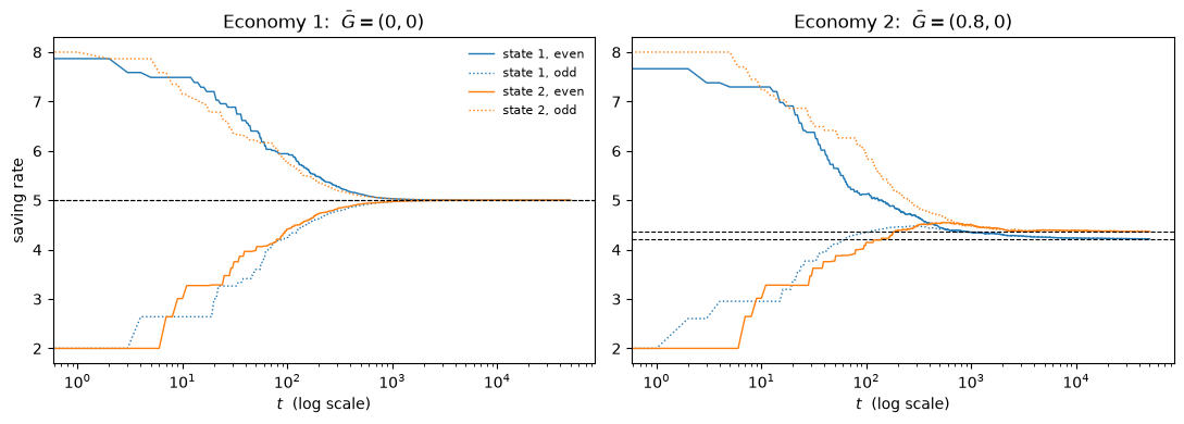
Fig. 85.1 Saving rates converge in both economies#
Both economies converge, and both classes of agent converge to the same rule even though neither learns from the other.
The dashed black lines are the equilibrium saving rates computed earlier from (85.5), objects that no agent in the simulation has access to.
rows = []
for T in (5_000, 50_000, 200_000):
    h1, _ = simulate(G1, P1, T=T, s0=start)
    h2, _ = simulate(G2, P2, T=T, s0=start)
    rows.append([T, *h1[-1].mean(axis=0), *h2[-1].mean(axis=0)])

pd.DataFrame(rows, columns=["T", "econ 1 state 1", "econ 1 state 2",
                            "econ 2 state 1", "econ 2 state 2"]).set_index("T").round(4)
| econ 1 state 1 | econ 1 state 2 | econ 2 state 1 | econ 2 state 2 | |
|---|---|---|---|---|
| T | ||||
| 5000 | 5.0004 | 5.0005 | 4.2551 | 4.3938 |
| 50000 | 5.0000 | 5.0000 | 4.2172 | 4.3708 |
| 200000 | 5.0000 | 5.0000 | 4.2106 | 4.3635 |
print(f"rational expectations: economy 1 = {np.round(s1, 4)}, economy 2 = {np.round(s2, 4)}")
rational expectations: economy 1 = [5. 5.], economy 2 = [4.2111 4.3637]
Convergence is slow — that is what a \(1/\tau\) gain buys you — but it is convergence, and to the right place.
85.3.4. How much do the agents have to be told?#
The specification above lets agents learn a separate saving rate for each level of the deficit.
In effect they are learning the policy function \(s = f(G)\) non-parametrically, state by state.
That is feasible here because there are only two states.
It has two drawbacks that Sargent emphasizes.
First, states that are rarely visited are learned about slowly, because the observations arrive slowly.
Exercise 85.1 makes this concrete.
Second, when the number of states is large, one parameter per state becomes unmanageable.
An econometrician’s response would be to impose a parametric form \(s = f(G, \theta)\) with \(\theta\) of low dimension and use every observation to estimate it, replacing (85.6) with a recursion in \(\theta\) driven by \(\partial U/\partial \theta\).
This buys speed at the cost of approximation: a parametric learning scheme can converge to a rational expectations equilibrium only if some member of the family \(f(\cdot, \theta)\) supports one.
Otherwise the best it can do is converge to an approximate equilibrium.
Note
This is the point at which models of learning and algorithms for computing equilibria become hard to tell apart.
Marcet’s method of parameterized expectations posits a parametric form for a conditional expectation, simulates, regresses realized outcomes on the parametric form to update the coefficients, and iterates.
Written recursively, that algorithm is a nonlinear-least-squares recursion of the same shape as (85.6).
Sargent’s summary: “Learning algorithms and equilibrium computation algorithms look like each other.”
An equilibrium computation is a centralized learning algorithm run by the modeller; a learning economy is a decentralized equilibrium computation run by the agents.
85.4. Part 2: a constant deficit and two steady states#
Now strip out the randomness.
Let the government finance a constant deficit \(G\) per young person, and let utility be \(\ln c_1 + \ln c_2\) as before.
With perfect foresight over the price level, the young save
where \(\pi_t\) is the gross inflation rate, the reciprocal of the return on currency.
The government’s budget constraint in real terms is \(h_t = h_{t-1}/\pi_{t-1} + G\), where \(h_t = m_t / p_t\), and equilibrium requires \(h_t = s_t\).
Eliminating \(h\) between these gives an autonomous difference equation in the inflation rate,
Stationary equilibria are the fixed points of \(g\), and since \(g\) is a hyperbola there are generically two of them.
We use the parameters of Marimon and Sunder [1993]’s “Economy 7C”: \(w_1 = 6\), \(w_2 = 1\), \(G = 1\).
w1_d, w2_d, G_d = 6.0, 1.0, 1.0
A1 = (w1_d + w2_d - 2*G_d) / w2_d
A2 = w1_d / w2_d

def g_map(π):
    return A1 - A2/π

π_low, π_high = np.sort(np.roots([1, -A1, A2]))
print(f"A1 = {A1},  A2 = {A2}")
print(f"stationary gross inflation rates: {π_low} and {π_high}")
print(f"   i.e. net inflation of {100*(π_low-1):.0f}% and {100*(π_high-1):.0f}% per period")
print(f"\nslope of g at the low  rate: {A2/π_low**2:.4f}   -> unstable under RE dynamics")
print(f"slope of g at the high rate: {A2/π_high**2:.4f}   -> stable under RE dynamics")
A1 = 5.0,  A2 = 6.0
stationary gross inflation rates: 2.0 and 3.0
   i.e. net inflation of 100% and 200% per period

slope of g at the low  rate: 1.5000   -> unstable under RE dynamics
slope of g at the high rate: 0.6667   -> stable under RE dynamics
There it is: the low-inflation stationary equilibrium is unstable under the rational expectations dynamics, and the high-inflation one is stable.
π_grid = np.linspace(1.35, 4.2, 400)

fig, ax = plt.subplots(figsize=(6.5, 5.5))
ax.plot(π_grid, g_map(π_grid), lw=1.6, label=r"$g(\pi) = A_1 - A_2/\pi$")
ax.plot(π_grid, π_grid, 'k--', lw=0.8, label="45 degree line")

# cobweb the RE dynamics away from the low steady state
π = π_low + 0.05
for _ in range(7):
    nxt = g_map(π)
    ax.plot([π, π], [π, nxt], color='C3', lw=0.9)
    ax.plot([π, nxt], [nxt, nxt], color='C3', lw=0.9)
    π = nxt

for p, name in [(π_low, "low"), (π_high, "high")]:
    ax.plot(p, p, 'ko', ms=6)
    ax.annotate(f"{name}\n$\\pi = {p:.0f}$", (p, p), textcoords="offset points",
                xytext=(10, -22), fontsize=9)
ax.set_xlabel(r"$\pi_t$")
ax.set_ylabel(r"$\pi_{t+1}$")
ax.legend(frameon=False, loc='upper left')
plt.show()
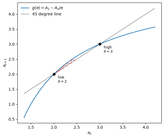
Fig. 85.2 Rational expectations inflation dynamics#
The red staircase starts just above the low-inflation steady state and marches away from it, straight to the high-inflation one.
def re_path(π0, T=25):
    path = [π0]
    for _ in range(T):
        nxt = g_map(path[-1])
        path.append(nxt if nxt > 0 else np.nan)
    return np.array(path)

pd.DataFrame({f"$\\pi_0 = {p}$": re_path(p) for p in (1.99, 2.01, 2.5, 4.0)}
             ).rename_axis("t").round(4).iloc[[0, 1, 2, 5, 10, 25]]
| $\pi_0 = 1.99$ | $\pi_0 = 2.01$ | $\pi_0 = 2.5$ | $\pi_0 = 4.0$ | |
|---|---|---|---|---|
| t | ||||
| 0 | 1.9900 | 2.0100 | 2.5000 | 4.0000 |
| 1 | 1.9849 | 2.0149 | 2.6000 | 3.5000 |
| 2 | 1.9772 | 2.0222 | 2.6923 | 3.2857 |
| 5 | 1.9187 | 2.0712 | 2.8836 | 3.0705 |
| 10 | 0.6693 | 2.3681 | 2.9830 | 3.0087 |
| 25 | NaN | 2.9961 | 3.0000 | 3.0000 |
Started fractionally below the low steady state the economy collapses (the price level implied by (85.8) goes negative); started fractionally above it, the economy converges to \(\pi = 3\).
This matters because of how the two equilibria rank.
The comparative statics of the low-inflation equilibrium are “classical”: raising the deficit \(G\) lowers \(A_1\), which raises the low stationary inflation rate.
The comparative statics of the high-inflation equilibrium are the reverse, because the economy is on the wrong side of an inflation-tax Laffer curve; see Exercise 85.3.
And the low-inflation equilibrium Pareto-dominates every other equilibrium of this model, stationary or not.
So the rational expectations dynamics repel the economy from the Pareto-optimal outcome, and most classical doctrine in monetary theory depends on selecting the equilibrium that those dynamics reject.
85.4.1. Least squares dynamics#
Marcet and Sargent [1989] studied a version of this economy in which agents do not have perfect foresight but instead run a regression.
Each period they regress the price level on its own lagged value and use the fitted slope as their forecast of gross inflation,
and then save \(s_t = (w_1 - w_2 \beta_t)/2\) according to (85.7).
Since \(\beta_t\) uses data through \(t-1\) only, there is no simultaneity: beliefs determine saving, saving determines the price level, and the new price level enters next period’s regression.
Writing \(\beta_t\) as
shows what the estimator is doing: it is a weighted average of past realized inflation rates, with weights proportional to \(p_{s-1}^2\).
That form is also what makes the recursion easy to compute.
The price level grows geometrically, so the two sums overflow quickly, but if we rescale both by the newest weight at each step everything stays of order one.
def ls_dynamics(π_init, T=3000):
    """
    Least squares dynamics.  Carries the two regression sums rescaled by the
    newest p^2, so nothing overflows even though the price level does not stop
    growing.  Returns (beliefs, realized inflation, survived?).
    """
    s_prev = (w1_d - w2_d*π_init) / 2
    num, den, π_last = π_init, 1.0, π_init
    betas, infl = [], []

    for t in range(T):
        β = num / den
        s_t = (w1_d - w2_d*β) / 2
        if s_t <= G_d or not np.isfinite(s_t):
            return np.array(betas), np.array(infl), False   # no positive price level
        π_t = s_prev / (s_t - G_d)                          # realized gross inflation
        num = num/π_last**2 + π_t
        den = den/π_last**2 + 1.0
        π_last, s_prev = π_t, s_t
        betas.append(β)
        infl.append(π_t)

    return np.array(betas), np.array(infl), True


rows = []
for π0 in (1.2, 1.5, 1.9, 2.0, 2.1, 2.5, 2.9, 3.0):
    b, infl, ok = ls_dynamics(π0)
    rows.append([π0, b[-1], infl[-1], "yes" if ok else "no"])

pd.DataFrame(rows, columns=["initial belief $\\pi_0$", "belief $\\beta_T$",
                            "realized $\\pi_T$", "survived"]).round(5)
| initial belief $\pi_0$ | belief $\beta_T$ | realized $\pi_T$ | survived | |
|---|---|---|---|---|
| 0 | 1.2 | 2.0 | 2.0 | yes |
| 1 | 1.5 | 2.0 | 2.0 | yes |
| 2 | 1.9 | 2.0 | 2.0 | yes |
| 3 | 2.0 | 2.0 | 2.0 | yes |
| 4 | 2.1 | 2.0 | 2.0 | yes |
| 5 | 2.5 | 2.0 | 2.0 | yes |
| 6 | 2.9 | 2.0 | 2.0 | yes |
| 7 | 3.0 | 2.0 | 2.0 | yes |
85.4.2. The stability reversal#
Least squares learning converges to the low-inflation equilibrium from every initial belief in the table, including from \(\pi_0 = 3.0\), which is the steady state that the rational expectations dynamics converge to.
fig, ax = plt.subplots(figsize=(8, 4.5))

for π0 in (1.5, 2.5, 3.0):
    _, infl, _ = ls_dynamics(π0, T=400)
    ax.plot(infl, color='C0', lw=1.2,
            label="least squares dynamics" if π0 == 1.5 else None)

for π0 in (2.05, 2.5, 4.0):
    ax.plot(re_path(π0, 400), color='C3', lw=1.2, ls='--',
            label="rational expectations dynamics" if π0 == 2.05 else None)

ax.axhline(π_low, color='k', lw=0.8, ls=':')
ax.axhline(π_high, color='k', lw=0.8, ls=':')
ax.annotate("low", (330, π_low + 0.04), fontsize=9)
ax.annotate("high", (330, π_high + 0.04), fontsize=9)
ax.set_xlim(0, 400)
ax.set_ylim(1.2, 4.2)
ax.set_xlabel("$t$")
ax.set_ylabel("gross inflation")
ax.legend(frameon=False)
plt.show()
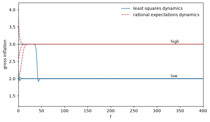
Fig. 85.3 Least squares and rational expectations inflation paths#
The two families of paths run in opposite directions.
The boundary is exact: least squares learning converges to \(\pi = 2\) from every initial belief up to and including \(\pi_0 = 3\), and above that the economy has no equilibrium price level at all.
lo, hi = 3.0, 3.2
for _ in range(40):                      # bisect for the edge of the basin
    mid = (lo + hi) / 2
    lo, hi = (mid, hi) if ls_dynamics(mid)[2] else (lo, mid)
print(f"least squares dynamics survive for initial beliefs up to {lo:.6f}")
print(f"the rational-expectations-stable steady state is      {π_high}")
least squares dynamics survive for initial beliefs up to 3.000000
the rational-expectations-stable steady state is      3.0
The steady state that the rational expectations dynamics single out as the stable one turns out to be precisely the edge of the basin of attraction of the learning dynamics toward the other one.
Why the reversal?
Under perfect foresight, a belief slightly above \(\pi_{\text{low}}\) is validated and amplified — the map \(g\) has slope \(1.5\) there.
Under least squares, beliefs are a weighted average of a long history of realized inflation rates, and that averaging drags the forecast back down.
The high steady state is stable for the forward-looking dynamics and repelling for the backward-looking ones.
Bruno and Fischer [1990] found the same reversal in a closely related model using Friedman-style adaptive expectations instead of least squares, so the result does not hinge on the details of the estimator.
85.4.3. Marimon and Sunder’s experiment#
Which set of dynamics describes people?
Marimon and Sunder [1993] built a laboratory economy to find out.
A fixed number of paying subjects were assigned roles as “young” and “old” in an implementation of exactly this model.
Each period the young submitted a schedule saying how much output they were willing to supply to the old for money at each price, and the experimenters cleared the market against the demand from the old and from the government.
Subjects temporarily on the sidelines played a forecasting game with its own cash prize, so the experiment produced a direct record of the price expectations driving the economy.
The session length was unknown to the subjects but governed by publicly announced rules that made the economy equivalent, from their point of view, to one that never ends.
Two findings matter here.
First, the experimental inflation paths were much better approximated by the least squares dynamics converging to the low stationary rate than by the rational expectations dynamics converging to the high one.
That pattern held across all of their economies.
Second, the sideliners’ forecast errors were comparable in size to those a least squares forecaster would have made using the same data.
The subjects were not doing something exotic, they were doing roughly what the adaptive model says.
The equilibrium that theory calls unstable is the one that both the algorithm and the humans select.
Note
Experimental evidence is not the only way to discriminate.
İmrohoroğlu [1993] estimated a rational expectations version of this model on German hyperinflation data and found the opposite: his estimated equilibrium slides along the bad side of the Laffer curve toward the high stationary rate, which is inconsistent with the equilibrium the adaptive dynamics select.
85.4.4. A warning#
It is tempting to conclude that adaptive dynamics reliably select the Pareto-superior equilibrium.
Sargent offers a counterexample, shown to him by Benjamin Bental, built from a special case of Brock [1974]’s money-in-the-utility-function model.
An infinitely lived household maximizes \(\sum_t \beta^t (\ln c_t + \gamma \ln(m_t/p_t))\) subject to a sequence of budget constraints, while the government finances a fixed expenditure \(g > 0\) by printing currency.
Under the parameter restriction \(\gamma(y - g) > g\) the model has a unique stationary equilibrium, with gross inflation
which has the classical property of rising with the deficit.
γ_b, β_b, y_b = 1.0, 1/1.05, 11.0

def brock_π(g):
    return ((y_b - g)*γ_b - β_b*g) / ((y_b - g)*γ_b - g)

pd.DataFrame({
    "$g$": [0.5, 1.0, 1.5, 2.0],
    "restriction $\\gamma(y-g) > g$": [γ_b*(y_b - g) > g for g in (0.5, 1.0, 1.5, 2.0)],
    "stationary $\\pi$": [brock_π(g) for g in (0.5, 1.0, 1.5, 2.0)],
    "return on currency $1/\\pi$": [1/brock_π(g) for g in (0.5, 1.0, 1.5, 2.0)],
}).round(5)
| $g$ | restriction $\gamma(y-g) > g$ | stationary $\pi$ | return on currency $1/\pi$ | |
|---|---|---|---|---|
| 0 | 0.5 | True | 1.00238 | 0.99762 |
| 1 | 1.0 | True | 1.00529 | 0.99474 |
| 2 | 1.5 | True | 1.00893 | 0.99115 |
| 3 | 2.0 | True | 1.01361 | 0.98658 |
But the model also has a continuum of non-stationary equilibria, indexed by initial price levels below the stationary one, in all of which the gross inflation rate converges to \(\beta\) — that is, the economy ends in deflation, with the return on currency approaching \(1/\beta = 1.05\) and real balances exploding.
These exist because the demand for currency implied by \(\gamma \ln(m/p)\) is so elastic with respect to the rate of return that the government can raise enough seigniorage to finance \(g\) even while paying interest on currency through deflation.
Applying least squares learning here selects the classical stationary equilibrium, just as in the overlapping generations model.
The difference is the welfare ranking: in the Brock model, the non-stationary equilibria all Pareto-dominate the classical stationary one that learning picks.
So least squares dynamics reliably select the classical equilibrium.
Whether that equilibrium is the good one is a separate question, and the answer depends on the model.
85.5. A government learning the Phillips curve#
The examples so far put adaptive households into a monetary economy.
We close with an application in which the adaptive agent is the government, learning an econometric relationship it can act on.
The environment is different from the overlapping generations model — it is a Phillips curve economy — but the machinery is the same: an agent runs a regression, acts on it, and thereby helps generate the very data it is fitting.
This example matters for a further reason.
It is the one in Sargent [1993] that most directly seeded later work: Sims [1988] and Chung [1990] studied it, and it led Sargent to the escape-dynamics model of Sargent [1999], The Conquest of American Inflation, which the Phillips curve lectures study in depth.
85.5.1. Two stories about post-war inflation#
There is a well-known account of the rise and fall of U.S. inflation after World War II.
In it, the private sector always had rational expectations and understood the natural-rate hypothesis, while the government, for a time, wrongly believed there was an exploitable Phillips curve, a lasting tradeoff between inflation and unemployment.
The government estimated Phillips curves on 1960s data, saw a tradeoff, and tried to buy lower unemployment with higher inflation.
The result was higher inflation with no lasting gain in employment: the Phillips curve shifted up adversely, as the natural-rate hypothesis says it must.
But there is a counter-story, told by economists who fit Phillips curves at the time.
They argued that their procedures were adaptive, that they detected the adverse shift quickly enough to give sound advice, and so need not have led the government astray.
The virtue of the model below is that a single specification nests both stories, with a parameter deciding which one plays out.
85.5.2. The model#
Inflation is decomposed into an expected and an unexpected part,
where \(g_{t-1}\) is the inflation the public expects (and which the government controls) and \(\eta_t\) is the public’s forecast error, orthogonal to earlier information.
The true Phillips curve is the natural-rate one: only the surprise \(\eta_t\) moves unemployment:
The government does not know this.
It believes unemployment depends on the level of inflation, and fits the non-expectational regression
Each period it minimizes \(\tfrac12 \mathbb{E}(U_t^2 + \pi_t^2)\) subject to its perceived model, which yields the myopic target
The system is self-referential: the government’s beliefs \(\alpha\) set its policy \(g\) through (85.12); the policy shapes the joint distribution of \((\pi, U)\); and that distribution is what the government’s regression (85.11) estimates.
U_star, θ_pc = 5.0, 1.0             # natural rate 5%, Phillips slope
σ_η, σ_u = 0.3, 0.3                 # inflation-surprise and unemployment shocks

def govt_target(α):
    "Government's myopic optimal target inflation."
    α0, α1 = α
    return -α0 * α1 / (1 + α1**2)
85.5.3. The consistent equilibrium#
A self-confirming, or consistent, equilibrium is a belief vector \(\alpha\) whose induced policy generates data whose regression returns the same \(\alpha\).
Under a constant policy \(g\), the surprise \(\eta_t\) is the only thing moving inflation around its mean, so the population regression of \(U\) on \(\pi\) has slope exactly \(-\theta\) and intercept \(U^* + \theta g\).
Solving that fixed point with the decision rule (85.12) gives Kydland and Prescott’s time-consistent outcome,
α_consistent = np.array([(1 + θ_pc**2) * U_star, -θ_pc])
g_consistent = θ_pc * U_star
print(f"consistent equilibrium beliefs α = {α_consistent},  target inflation g = {g_consistent}")
print(f"optimal (Ramsey) outcome:                                  target inflation g = 0")
consistent equilibrium beliefs α = [10. -1.],  target inflation g = 5.0
optimal (Ramsey) outcome:                                  target inflation g = 0
This is the inflation bias.
The government inflates at rate \(\theta U^*\) and gets nothing for it: because only surprises move unemployment, average unemployment is \(U^*\) either way.
- Had the government understood the true model (85.10), it would have chosen \(g = 0\)
the same unemployment with none of the inflation.
85.5.4. Constant-coefficient beliefs: learning the inflation bias#
Suppose the government believes its coefficients are constant and estimates them by least squares, updating a little each period.
The deterministic path that least squares learning follows on average — its mean dynamics — moves beliefs toward the regression their current policy would induce.
def induced_beliefs(α):
    "The OLS fit that the current beliefs' policy would induce in a stationary sample."
    g = govt_target(α)
    return np.array([U_star + θ_pc * g, -θ_pc])          # slope is exactly -θ

def mean_dynamics(α0=(0.0, 0.0), lr=0.2, T=60):
    α = np.array(α0, float)
    path = np.empty((T, 3))
    for t in range(T):
        α = α + lr * (induced_beliefs(α) - α)
        path[t] = [α[0], α[1], govt_target(α)]
    return path

path = mean_dynamics()

fig, ax = plt.subplots(figsize=(7.5, 4))
ax.plot(path[:, 2], 'C0', lw=1.6, label="target inflation $g$")
ax.plot(path[:, 0], 'C1', lw=1.2, label=r"belief $\alpha_0$")
ax.plot(path[:, 1], 'C2', lw=1.2, label=r"belief $\alpha_1$")
ax.axhline(g_consistent, color='C0', ls='--', lw=0.8)
ax.set_xlabel("iteration")
ax.legend(frameon=False)
plt.show()
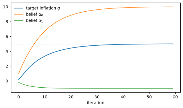
Fig. 85.4 Least squares learning converges to the inflation bias#
Least squares learning walks the government straight into the consistent equilibrium: beliefs settle at \(\alpha = ((1+\theta^2)U^*, -\theta)\) and target inflation at \(\theta U^* = 5\).
The government keeps inflating, period after period, at a rate that buys it nothing, because its own policy keeps producing data that confirm the tradeoff it believes in.
85.5.5. Random-coefficient beliefs: escaping toward the optimum#
Sims [1988] and Chung [1990] then asked what happens if the government is less sure its coefficients are constant.
They let the government suspect the coefficients drift — a random walk in \(\alpha\) — and estimate them with a Kalman filter, which discounts old data in favor of recent data.
That is a constant-gain algorithm: instead of a \(1/t\) gain that eventually freezes the estimates, it keeps a fixed gain forever, so the government never stops paying attention to what just happened.
def constant_gain(T=40_000, gain=0.02, seed=1):
    "Government estimates a drifting-coefficient Phillips curve; returns target inflation g_t."
    rng = np.random.default_rng(seed)
    α = α_consistent.copy()                              # start at the inflation bias
    R = np.eye(2)
    g_path = np.empty(T)
    for t in range(T):
        g = govt_target(α)
        η = σ_η * rng.standard_normal()
        π = g + η
        U = U_star - θ_pc * η + σ_u * rng.standard_normal()   # true Phillips curve
        x = np.array([1.0, π])
        R = R + gain * (np.outer(x, x) - R)
        α = α + gain * np.linalg.solve(R, x * (U - x @ α))
        g_path[t] = g
    return g_path

g_path = constant_gain()

fig, ax = plt.subplots(figsize=(9, 4))
ax.plot(g_path, lw=0.5)
ax.axhline(g_consistent, color='C3', ls='--', lw=1, label="consistent equilibrium (inflation bias)")
ax.axhline(0, color='C2', ls=':', lw=1, label="Ramsey / zero inflation")
ax.set_xlabel("$t$")
ax.set_ylabel("target inflation $g_t$")
ax.legend(frameon=False)
plt.show()
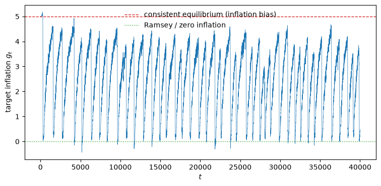
Fig. 85.5 Constant-gain learning and recurrent escapes to zero inflation#
The constant-gain government does not settle at the inflation bias.
It climbs toward it, then abruptly escapes toward zero inflation, then drifts back up, then escapes again, in a recurring sawtooth.
The mechanism is the one Sims and Chung identified.
Because the government discounts old data, a run of observations in which inflation surprises are small and unemployment stays near \(U^*\) regardless of inflation quickly persuades it that the tradeoff is not there, and it stops exploiting a tradeoff it no longer believes in, dropping inflation toward zero.
The willingness to entertain drifting coefficients lets the government learn the truth of the natural-rate hypothesis without having to sit through a long inflation to do it.
How often the escapes happen depends on the gain — the government’s degree of doubt about its own model — which is exactly the parameter Sims [1988] found to select between the two stories.
A small gain keeps the economy near the inflation bias; a larger gain sends it toward the optimum more often (Exercise 85.4).
85.5.6. From escape dynamics to the Conquest of American Inflation#
The two regimes are formalizations of the two stories we began with.
The consistent-equilibrium path is the natural-rate story: a government that trusts its mis-specified model inflates and stays stuck.
The escaping path is the counter-story: a government alert to model change detects the poor tradeoff and backs away from it.
This is the seed of a large literature.
Sims [1988] and Chung [1990] showed both that the model could nest the two stories and — in Chung’s case — that it could be econometrically estimated on post-war U.S. data, imputing a genuine estimation procedure to the government inside the model.
Their work led Sargent [1999] to the escape-route model of The Conquest of American Inflation, in which recurrent escapes from the high-inflation Nash equilibrium toward the Ramsey outcome offer a theory of how U.S. inflation was actually conquered in the early 1980s.
The QuantEcon lectures Escaping Nash Inflation and Adaptive Learning and Escape Dynamics develop that model and its escape dynamics in full; the sawtooth above is a first glimpse of what they study.
85.6. Concluding remarks#
Part 1 showed that a system of adaptive agents can find a rational expectations equilibrium it was never told about, and made visible how much the complexity of the environment governs the speed: a rare deficit state is learned about slowly, and a large state space forces a parametric shortcut that may put the equilibrium out of reach entirely.
Part 2 showed something stronger.
Where the model has two equilibria, the learning dynamics do not merely find one; they systematically pick out the one that the rational expectations dynamics reject, and laboratory subjects go the same way.
That is the best case in Sargent [1993] for treating adaptive dynamics as an equilibrium selection device.
The Brock counterexample marks its limit.
The selection is a fact about the algorithm, not a welfare theorem, and Sargent is candid about the resulting discomfort:
I know that it is inconsistent to doubt the real-time dynamics but keep the equilibria selected by them. I confess that my affection for the selection performed in the monetary models described in Chapter 6 is partly driven by my prior conviction that the selected equilibria seem sensible to me.
The Phillips curve application sharpened the point in two ways.
It showed that which learning scheme finds the good outcome is model-dependent: here least squares walks into the bad equilibrium, and it is the constant-gain government — the one that never stops doubting — that escapes toward the good one.
And it turned the gain into the object of interest, foreshadowing the escape-dynamics research of Sargent [1999] taken up in Escaping Nash Inflation and Adaptive Learning and Escape Dynamics.
Money as a Medium of Exchange among Artificially Intelligent Agents takes the selection idea in a different direction, into a setting where the competing equilibria are not high and low inflation but different monetary institutions: which good becomes money.
85.7. Exercises#
Exercise 85.1
Because agents learn a separate saving rate for each deficit state, they can only learn about a state as fast as that state occurs.
Compare two economies with \(\bar G = (0.8, 0)\) that differ only in the transition matrix: one where the two states are equally likely, and one where the high-deficit state is rare.
For each, compute the stationary equilibrium, run the learning simulation, and report how far each state’s learned saving rate is from its target along with how often that state was visited.
Solution
G_ex = np.array([0.8, 0.0])
cases = {"equally likely": np.array([[0.5, 0.5], [0.5, 0.5]]),
         "high deficit rare": np.array([[0.5, 0.5], [0.03, 0.97]])}

rows = []
for name, P in cases.items():
    s_star, _ = stationary_equilibrium(G_ex, P)
    ergodic = qe.MarkovChain(P).stationary_distributions[0]
    hist, _ = simulate(G_ex, P, T=30_000, s0=start)
    learned = hist[-1].mean(axis=0)
    for k in (0, 1):
        rows.append([name, k+1, ergodic[k], s_star[k], learned[k],
                     abs(learned[k] - s_star[k])])

pd.DataFrame(rows, columns=["chain", "state", "ergodic prob.",
                            "equilibrium $s_i$", "learned $s_i$", "error"]).round(4)
| chain | state | ergodic prob. | equilibrium $s_i$ | learned $s_i$ | error | |
|---|---|---|---|---|---|---|
| 0 | equally likely | 1 | 0.5000 | 4.4965 | 4.5031 | 0.0066 |
| 1 | equally likely | 2 | 0.5000 | 4.4965 | 4.5006 | 0.0041 |
| 2 | high deficit rare | 1 | 0.0566 | 4.6828 | 4.6994 | 0.0167 |
| 3 | high deficit rare | 2 | 0.9434 | 4.9646 | 4.9662 | 0.0016 |
When the two states are equally likely the two saving rules are learned about equally well.
When the high-deficit state occurs only about six percent of the time, the error in its rule is an order of magnitude larger than the error in the rule for the common state, even though both have had 30,000 periods of calendar time to settle.
Sargent’s comment is worth keeping in mind: in terms of unconditional expected utility, failing to learn what to do in a rarely visited state may cost very little.
The cost of slow learning is not proportional to the size of the error.
Note also that changing the transition matrix changes the equilibrium itself — beliefs about the persistence of deficits feed straight into (85.5) — so the comparison has to be against a separately recomputed target for each chain.
Exercise 85.2
The gain sequence \(\gamma_\tau = 1/\tau\) is what makes (85.6) converge.
An agent who suspected the environment might be drifting would use a constant gain instead, weighting recent experience more heavily forever.
Modify the simulation to use a constant gain and describe what happens to the limiting behavior of the saving rules.
Compare gains of \(0.02\) and \(0.005\) against the \(1/\tau\) benchmark.
Solution
def simulate_constant_gain(G, P, gain, T=30_000, s0=None, seed=0, band=0.4):
    rng = np.random.default_rng(seed)
    n = len(G)
    s = np.array(s0, float)
    M = np.array([[U_double(s[j, k], 1.0) for k in range(n)] for j in range(2)])
    floor = G/N + band
    hist = np.empty((T, 2, n))
    i, prev = 0, None
    for t in range(T):
        j = t % 2
        s_t = s[j, i]
        if prev is not None:
            j_p, i_p, s_p = prev
            R = (N*s_t - G[i]) / (N*s_p)
            M[j_p, i_p] += gain * (U_double(s_p, R) - M[j_p, i_p])
            step = gain * U_prime(s_p, R) / M[j_p, i_p]
            s[j_p, i_p] = np.clip(s[j_p, i_p] - step, floor[i_p], w1 - 0.4)
        prev = (j, i, s_t)
        hist[t] = s
        i = rng.choice(n, p=P[i])
    return hist

rows = []
for label, hist in [("gain = 0.02", simulate_constant_gain(G2, P2, 0.02, s0=start)),
                    ("gain = 0.005", simulate_constant_gain(G2, P2, 0.005, s0=start)),
                    ("gain = 1/τ", simulate(G2, P2, T=30_000, s0=start)[0])]:
    tail = hist[-5_000:].mean(axis=1)        # average the two classes
    rows.append([label, *tail.mean(axis=0), *tail.std(axis=0)])

pd.DataFrame(rows, columns=["", "mean $s_1$", "mean $s_2$",
                            "s.d. $s_1$", "s.d. $s_2$"]).set_index("").round(5)
| mean $s_1$ | mean $s_2$ | s.d. $s_1$ | s.d. $s_2$ | |
|---|---|---|---|---|
| gain = 0.02 | 4.20862 | 4.36167 | 0.04089 | 0.04015 |
| gain = 0.005 | 4.20937 | 4.34929 | 0.01391 | 0.02159 |
| gain = 1/τ | 4.22312 | 4.37010 | 0.00057 | 0.00098 |
fig, ax = plt.subplots(figsize=(8, 4))
for gain, colour in [(0.02, 'C1'), (0.005, 'C2')]:
    h = simulate_constant_gain(G2, P2, gain, s0=start)
    ax.plot(h[:, 0, 0], color=colour, lw=0.7, label=f"gain = {gain}")
h, _ = simulate(G2, P2, T=30_000, s0=start)
ax.plot(h[:, 0, 0], color='C0', lw=1.2, label=r"gain = $1/\tau$")
ax.axhline(s2[0], color='k', lw=0.8, ls='--', label="equilibrium")
ax.set_xlim(0, 30_000)
ax.set_ylim(3.8, 5.0)
ax.set_xlabel("$t$")
ax.set_ylabel("saving rate, state 1")
ax.legend(frameon=False, fontsize=9)
plt.show()
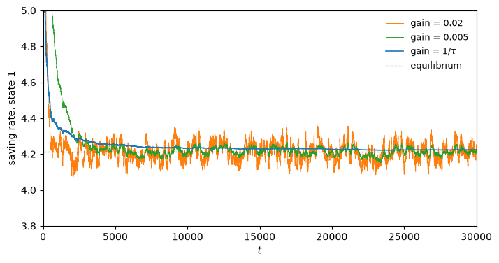
The constant-gain rules do not converge.
They settle into a neighborhood of the equilibrium and then keep rattling around inside it forever, because each new observation is always given the same weight and so never stops moving the estimate.
Shrinking the gain tightens the band but does not eliminate it.
Only a gain that declines to zero — like \(1/\tau\) — delivers convergence to a point, which is why the convergence theorems for these systems all require it.
What the constant-gain agent buys in exchange is adaptability: if the deficit process were to change, the \(1/\tau\) agent would barely notice, while the constant-gain agent would track the change.
That trade-off reappears throughout this literature.
Exercise 85.3
The claim that the high-inflation steady state sits on “the wrong side of a Laffer curve” can be made precise.
In a stationary equilibrium with gross inflation \(\pi\), real balances are \(h = (w_1 - w_2\pi)/2\) and the government collects seigniorage \(h(1 - 1/\pi)\).
Plot seigniorage as a function of \(\pi\), mark the two stationary equilibria, and use the picture to explain why raising \(G\) raises the low stationary inflation rate but lowers the high one, and what happens when \(G\) gets too large.
Solution
def seigniorage(π):
    return (w1_d - w2_d*π)/2 * (1 - 1/π)

π_grid = np.linspace(1.01, 5.5, 500)
peak = π_grid[np.argmax(seigniorage(π_grid))]

fig, ax = plt.subplots(figsize=(7.5, 4.5))
ax.plot(π_grid, seigniorage(π_grid), lw=1.6)
for G_try, style in [(1.0, '-'), (1.03, '--'), (1.0505, ':')]:
    ax.axhline(G_try, color='C3', lw=0.9, ls=style, label=f"$G = {G_try}$")
ax.plot([π_low, π_high], [seigniorage(π_low), seigniorage(π_high)], 'ko', ms=6)
ax.axvline(peak, color='gray', lw=0.8, ls=':')
ax.set_xlabel(r"gross inflation $\pi$")
ax.set_ylabel("seigniorage")
ax.set_ylim(0, 1.5)
ax.legend(frameon=False)
plt.show()

print(f"peak of the Laffer curve at π = {peak:.4f}, raising {seigniorage(peak):.4f}")
print(f"the two steady states raise {seigniorage(π_low):.4f} and {seigniorage(π_high):.4f}")
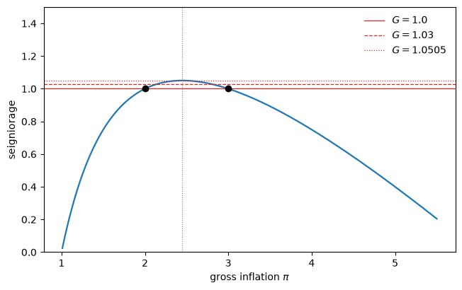
peak of the Laffer curve at π = 2.4497, raising 1.0505
the two steady states raise 1.0000 and 1.0000
The two stationary equilibria are the two inflation rates at which the inflation-tax Laffer curve crosses the required revenue \(G\), one on each side of the peak.
The low one sits on the rising branch, so financing a larger deficit there requires more inflation: the classical comparative static.
The high one sits on the falling branch, where more inflation raises less revenue, so a larger deficit is financed by a lower stationary inflation rate, the anti-classical comparative static that makes the high equilibrium so awkward.
As \(G\) rises the horizontal line moves up and the two intersections converge.
Past the peak of the curve there is no stationary equilibrium at all: the deficit exceeds the maximum revenue the inflation tax can raise.
rows = []
for G_try in (0.8, 1.0, 1.04, 1.05, 1.0505, 1.06):
    A1_try = (w1_d + w2_d - 2*G_try)/w2_d
    disc = A1_try**2 - 4*A2
    if disc < 0:
        rows.append([G_try, np.nan, np.nan, "none"])
    else:
        r = np.sort(np.roots([1, -A1_try, A2]))
        rows.append([G_try, r[0], r[1], "two"])

pd.DataFrame(rows, columns=["$G$", "low $\\pi$", "high $\\pi$",
                            "stationary equilibria"]).round(4)
| $G$ | low $\pi$ | high $\pi$ | stationary equilibria | |
|---|---|---|---|---|
| 0 | 0.8000 | 1.5642 | 3.8358 | two |
| 1 | 1.0000 | 2.0000 | 3.0000 | two |
| 2 | 1.0400 | 2.2328 | 2.6872 | two |
| 3 | 1.0500 | 2.4000 | 2.5000 | two |
| 4 | 1.0505 | 2.4424 | 2.4566 | two |
| 5 | 1.0600 | NaN | NaN | none |
The two roots move toward each other as \(G\) rises and collide at \(G \approx 1.0505\), after which the model has no stationary equilibrium at all.
That number is not a coincidence.
Setting the discriminant of (85.8)’s fixed-point equation to zero gives a double root at \(\pi = \sqrt{A_2} = \sqrt{w_1/w_2}\), and the deficit at which it occurs is exactly the peak of the Laffer curve computed above.
G_max = (w1_d + w2_d - 2*np.sqrt(A2)*w2_d) / 2
print(f"roots collide at G       = {G_max:.6f},  where π = √(w1/w2) = {np.sqrt(A2):.6f}")
print(f"peak of the Laffer curve = {seigniorage(np.sqrt(A2)):.6f}  at π = {np.sqrt(A2):.6f}")
roots collide at G       = 1.050510,  where π = √(w1/w2) = 2.449490
peak of the Laffer curve = 1.050510  at π = 2.449490
The largest deficit the government can finance is the maximum of the inflation tax, and at that deficit the two stationary equilibria have merged into one.
Exercise 85.4
In the Phillips curve application, the constant-gain government escapes toward zero inflation, and the lecture claims that how often it escapes depends on the gain, the government’s degree of doubt about its own model.
Make the claim quantitative.
For a range of gains, simulate the constant-gain economy and measure both the average target inflation and the fraction of time spent near the Ramsey outcome (say, \(g_t < 1\)).
Which way does more doubt push the economy, and how does this connect to the two stories about post-war inflation?
Solution
rows = []
for gain in (0.005, 0.01, 0.02, 0.04, 0.08):
    tails = [constant_gain(T=30_000, gain=gain, seed=s)[-20_000:] for s in range(4)]
    mean_g = np.mean([g.mean() for g in tails])
    near_ramsey = np.mean([np.mean(g < 1) for g in tails])
    rows.append([gain, mean_g, near_ramsey])

pd.DataFrame(rows, columns=["gain", "mean target inflation", "fraction of time $g < 1$"]
             ).set_index("gain").round(3)
| mean target inflation | fraction of time $g < 1$ | |
|---|---|---|
| gain | ||
| 0.005 | 3.221 | 0.121 |
| 0.010 | 2.886 | 0.148 |
| 0.020 | 2.485 | 0.174 |
| 0.040 | 2.174 | 0.189 |
| 0.080 | 1.820 | 0.210 |
More doubt — a larger gain — pushes the economy away from the inflation bias and toward the optimum: mean inflation falls and the economy spends a larger fraction of its time near the Ramsey outcome.
The intuition is that a higher gain discounts old data more heavily, so the government reacts faster to the run of observations that reveals the tradeoff to be illusory, and escapes sooner and more often.
This is exactly the parameter Sims [1988] found to select between the two stories.
A government confident in its constant-coefficient model (small gain) is the natural-rate story’s government, stuck inflating; a government alert to model change (large gain) is the counter-story’s, detecting the poor tradeoff and stepping away from it.
The same gain reappears as the central object in Sargent [1999], where the rate of escape from the high-inflation equilibrium governs how quickly an inflation can be conquered.