89. Money as a Medium of Exchange among Artificially Intelligent Agents#
89.1. Overview#
Kiyotaki and Wright [Kiyotaki and Wright, 1989] studied an economy in which there is no double coincidence of wants.
Trade can occur only if some good is accepted not because it is wanted, but because it can be passed along later.
A good that plays that role is a medium of exchange.
Kiyotaki and Wright characterized stationary Nash equilibria of such an economy under the assumption that agents are fully rational: agents know the distribution of goods across their trading partners and best-respond to it.
Marimon, McGrattan and Sargent [Marimon et al., 1990] asked a different question.
Suppose we drop rationality altogether and put in its place a collection of artificially intelligent agents who begin with arbitrary, even random, rules of thumb, and who adapt those rules only by keeping score of what has paid off in the past.
Will such agents learn to use a medium of exchange?
And when the rational-expectations model has more than one equilibrium, which one, if any, will emerge?
The learning device that Marimon, McGrattan and Sargent used is John Holland’s classifier system [Holland, 1975, Holland et al., 1986]: a population of if-then rules, an auction that decides which rule acts, and an accounting system that credits rules that lead to good outcomes and debits rules that lead to bad ones.
Optionally, a genetic algorithm breeds new rules and retires old ones.
This lecture rebuilds their computational experiments.
The main findings that we shall reproduce are:
Starting from a complete enumeration of rules with equal strengths, or even from randomly generated rules, holdings and trading patterns converge to a stationary Nash equilibrium of the Kiyotaki-Wright model.
When the Kiyotaki-Wright model has both a fundamental and a speculative equilibrium, the artificially intelligent agents select the fundamental one – the one in which the good with the lowest storage cost circulates as money.
An intrinsically worthless, costlessly stored object – fiat money – is accepted in trade by agents who have to discover its usefulness for themselves.
The same machinery works in an economy with five goods and five types for which the authors had no analytical characterization of equilibrium: the algorithm is used as an equilibrium-discovery device.
Let’s start with some imports.
import numpy as np
import pandas as pd
import matplotlib.pyplot as plt
from dataclasses import dataclass
89.2. The Kiyotaki-Wright environment#
There are three types of agents, indexed by \(i = 1, 2, 3\), and three goods, indexed by \(k = 1, 2, 3\).
A type \(i\) agent derives utility only from consuming good \(i\).
He has a technology for producing good \(i^*\), where \(i^* \neq i\).
In Kiyotaki and Wright’s model A, the production pattern is the “Wicksell triangle”
type \(i\) |
produces \(i^*\) |
consumes |
|---|---|---|
1 |
2 |
1 |
2 |
3 |
2 |
3 |
1 |
3 |
so there is no double coincidence of wants: the agent who has what you want never wants what you have.
All goods are indivisible and each agent can store exactly one unit of exactly one good from one period to the next.
Storing good \(k\) for one period costs \(s_k\), with
There are equal numbers \(A_i\) of agents of each type, so \(A = 3 A_i\) in total.
Each period every agent is randomly matched with exactly one other agent, without regard to type.
Write \(x_{at}\) for the good that agent \(a\) carries into date \(t\) and \(\rho_t(a)\) for the agent with whom \(a\) is matched.
The pre-trade state of agent \(a\) is the pair
Each period each agent makes two decisions in sequence.
First, having seen \(z_{at}\), he decides whether to propose a trade,
Trade occurs if and only if \(\lambda_{at} \lambda_{\rho_t(a)t} = 1\), so post-trade holdings are
Second, he decides whether to consume what he is left holding,
If he consumes he immediately produces good \(f(a) = i^*\) and carries that into \(t+1\).
Hence
The one-period net payoff is
where \(u_i(k) = u_i > 0\) if \(k = i\) and \(u_i(k) = 0\) otherwise.
Note that an agent is permitted to consume a good he does not want; he simply gets zero utility from it while still producing and paying to store \(f(a)\).
Not consuming is not free either – it costs \(s(x^+_{at})\).
Learning which of these to do is part of the problem.
Note
Kiyotaki and Wright ranked payoff streams by expected discounted utility.
Marimon, McGrattan and Sargent instead assume that each agent cares about his long-run average utility.
This matters: as we shall see, it is the reason the accounting system inside a classifier system is built out of running averages.
89.2.1. Two equilibria#
Since agents’ payoffs depend on what other agents do, the model can have more than one stationary equilibrium.
Kiyotaki and Wright characterize equilibria by a set of probabilities, of which the most useful for us is
In the fundamental equilibrium, good 1 – the cheapest to store – is the general medium of exchange:
type 1 agents always hold good 2 (which they produce) and trade it for good 1;
type 3 agents always hold good 1 and trade it for good 3;
type 2 agents hold good 1 half the time and good 3 half the time.
So the equilibrium holding probabilities are
\(k=1\) |
\(k=2\) |
\(k=3\) |
|
|---|---|---|---|
\(i=1\) |
0 |
1 |
0 |
\(i=2\) |
0.5 |
0 |
0.5 |
\(i=3\) |
1 |
0 |
0 |
Type 2 agents accept good 1 even though they never consume it: they use it as money.
In the speculative equilibrium, type 1 agents additionally accept good 3 – the most expensive good to store – because they expect to trade it away quickly for good 1.
Kiyotaki and Wright show that, in the limit as the discount rate goes to zero, the fundamental equilibrium is the unique stationary equilibrium if
and the speculative equilibrium is the unique one when the inequality is reversed.
Raising \(u_1\) enough therefore flips the model’s prediction from fundamental to speculative.
Economy A2 below does exactly that, and it is a good test of whether adaptive agents track the rational-expectations prediction.
89.3. Classifier systems#
An agent is not endowed with a strategy.
He is endowed with a population of candidate rules and a way of keeping score.
A classifier is a string in the trinary alphabet \(\{0, 1, \#\}\) split into a condition and an action, where \(\#\) means “don’t care”.
[Goldberg, 1989] is a book-length treatment of classifier systems and genetic algorithms.
Goods are encoded in binary and conditions in trinary, so with three goods two positions suffice:
code |
meaning |
|---|---|
|
good 1 |
|
good 2 |
|
good 3 |
|
not good 1 |
|
not good 2 |
|
any good |
An exchange classifier is a string of length 7: two positions for own holding, two for the partner’s holding, and a final binary digit for the action (\(1\) = propose trade, \(0\) = refuse).
For example
1 0 0 0 1   ->  1     "if I hold good 1 and my partner holds good 3, propose to trade"
1 0 # #     ->  0     "if I hold good 1, refuse to trade with anyone"
There are \(6 \times 6 \times 2 = 72\) distinct exchange classifiers, which is a complete enumeration of all rules definable on the state \(z_{at}\).
A consumption classifier is a string of length 4: two positions for the post-trade holding \(x^+_{at}\) and one action digit (\(1\) = consume).
There are \(6 \times 2 = 12\) of these.
89.3.1. The auction#
Attached to classifier \(e\) at date \(t\) is a strength \(S^a_e(t)\).
Given the state \(z_{at}\), let
be the set of classifiers whose conditions are satisfied.
The classifier that acts is the strongest matched one,
and the consumption classifier is chosen the same way from \(M_c(z_{at})\).
89.3.2. The bucket brigade#
Strengths are updated by a system of internal payments that Holland calls a bucket brigade.
Only the classifier that wins an auction changes its strength, so we attach to each classifier a counter \(\tau^a_e(t)\) recording the number of auctions it has won up to \(t\), initialized at 1.
A matched classifier \(e\) bids the fraction
of its strength, and similarly \(b_2(c) = b_{21} + b_{22}\sigma_c\) for consumption classifiers.
Because \(\sigma_e\) rises with specificity, specific rules outbid general ones of equal strength.
Payments flow as follows.
The external payoff \(U_a(\gamma_t)\) goes to the winning consumption classifier at \(t\).
The winning consumption classifier at \(t\) pays its bid to the winning exchange classifier at \(t\), which created the state that gave it a chance to act.
The winning exchange classifier at \(t\) pays its bid to the winning consumption classifier at \(t-1\), which set up the state \(z_{at}\).
This chain is what transmits the reward for consuming backwards to the trades that made consumption possible.
The resulting laws of motion are
where \(I^a_e(t)\) and \(I^a_c(t)\) are indicators for winning the auction at \(t\).
The timing in (89.6) is worth reading carefully, because it is what carries reward across periods.
The consumption classifier updated at date \(t\) is the one that won at \(t-1\): it collects the external payoff its own decision earned, and it collects the bid \(b_1(e)S_e\) from the exchange classifier winning now, because that is the classifier whose opportunity to act it created.
The exchange classifier, in turn, is paid within the period by the consumption classifier that follows it.
So each bid travels one step back along the chain
and a payoff collected at consumption seeps backwards, one link per payment, to the trades that made it possible.
An exchange classifier that proposes a trade which is not reciprocated is not charged and its counter does not advance: the agent learns nothing from an offer that was refused.
Note
Equations (89.6)-(89.7) make strength a cumulative average of past net receipts rather than a cumulative total, which is what Holland’s original specification used.
This is the innovation that makes strengths converge.
With \(1/\tau\) gains these are stochastic approximation recursions, so any limit point must satisfy
Marimon, McGrattan and Sargent define a set of strengths solving these equations to be stationary, and a stationary Nash equilibrium to be supported when the rules that win auctions at stationary strengths are exactly the rules that support equilibrium behavior.
All agents of a given type share one classifier system, as in the paper; this economizes on computation at the cost of making all type \(i\) agents experiment simultaneously.
89.4. Implementation#
We store a population of classifiers as a set of parallel NumPy arrays rather than as a list of objects, which lets us find all matched rules with a single vectorized comparison.
The wildcard \(\#\) is represented by \(-1\).
WILD = -1

# binary codes for goods, one row per good
CODES = {
    3: np.array([[1, 0], [0, 1], [0, 0]]),
    4: np.array([[1, 0], [0, 1], [0, 0], [1, 1]]),          # good 4 = fiat money
    5: np.array([[1, 0, 0], [0, 1, 0], [0, 0, 1],
                 [1, 1, 0], [1, 0, 1]]),
}

# the six conditions expressible with two trits (see the table above)
CONDS_2 = np.array([[1, 0], [0, 1], [0, 0],
                    [0, WILD], [WILD, 0], [WILD, WILD]])


def rule_string(cond, action):
    "Print a classifier the way the paper does."
    body = ''.join('#' if b == WILD else str(int(b)) for b in cond)
    return f"{body} -> {int(action)}"
class Rules:
    """
    A population of classifiers held as parallel arrays.

    cond[i]     condition part of rule i, entries in {0, 1, WILD}
    action[i]   action part of rule i, in {0, 1}
    strength[i] S_i, a running average of net receipts
    used[i]     the counter tau_i, initialized at 1
    traded[i]   number of times rule i actually executed a trade

    """

    def __init__(self, cond, action, strength=None):
        self.cond = np.asarray(cond, dtype=np.int64)
        self.action = np.asarray(action, dtype=np.int64)
        n = len(self.action)
        self.strength = (np.zeros(n) if strength is None
                         else np.asarray(strength, float).copy())
        self.used = np.ones(n, dtype=np.int64)
        self.traded = np.zeros(n, dtype=np.int64)

    @property
    def n(self):
        return len(self.action)

    @property
    def length(self):
        return self.cond.shape[1]

    def matched(self, state):
        "Boolean mask of rules whose condition is satisfied by state."
        return np.all((self.cond == WILD) | (self.cond == state), axis=1)

    def specificity(self, i):
        "sigma_i = 1 / (1 + number of wildcards)."
        return 1.0 / (1.0 + np.count_nonzero(self.cond[i] == WILD))

    def replace(self, i, cond, action, strength, used=1, traded=0):
        "Overwrite rule i."
        self.cond[i] = cond
        self.action[i] = action
        self.strength[i] = strength
        self.used[i] = used
        self.traded[i] = traded
A complete enumeration pairs every condition with both actions.
A random population draws conditions and actions uniformly, which is how the incomplete-enumeration economies start.
def complete_rules(pair):
    "All two-trit rules; pair=True for exchange rules, False for consumption rules."
    if pair:
        conds = np.array([np.concatenate([a, b])
                          for a in CONDS_2 for b in CONDS_2])
    else:
        conds = CONDS_2.copy()
    return Rules(np.repeat(conds, 2, axis=0), np.tile([0, 1], len(conds)))


def random_rules(n, length, rng):
    return Rules(rng.integers(-1, 2, size=(n, length)),
                 rng.integers(0, 2, size=n),
                 rng.random(n) * 0.1)
The auction (89.5) picks the strongest matched rule, with ties broken by position.
def auction(rules, state):
    "Index of the strongest rule matching state, or -1 if none matches."
    idx = np.flatnonzero(rules.matched(state))
    if idx.size == 0:
        return -1, idx
    return idx[np.argmax(rules.strength[idx])], idx
Two operators are needed even without a genetic algorithm.
Creation fires when the current state matches no rule at all: a redundant or weak rule is overwritten by one whose condition is exactly the state just observed, with a randomly drawn action.
Diversification fires when every matched rule calls for the same action: a rule with the opposite action is planted so that the alternative can be tried and scored.
Both keep the population size constant.
def create(rules, state, rng):
    "No rule matches state, so overwrite the weakest of the most redundant rules."
    groups = {}
    for i in range(rules.n):
        groups.setdefault(tuple(rules.cond[i]), []).append(i)
    biggest = max(groups.values(), key=len)
    group = biggest if len(biggest) > 1 else range(rules.n)
    j = min(group, key=lambda i: rules.strength[i])
    rules.replace(j, state, rng.integers(0, 2), rules.strength.mean())
    return j


def diversify_simple(rules, matches):
    "If every matched rule takes the same action, plant the opposite action."
    if len(set(rules.action[matches])) > 1:
        return
    weak = matches[np.argmin(rules.strength[matches])]
    rules.replace(weak, rules.cond[weak], 1 - rules.action[matches[0]],
                  rules.strength[matches].mean())
89.4.1. Describing an economy#
An Economy collects the parameters of the physical environment together with the settings
of the learning algorithm.
The field method selects one of the three programs used in the paper:
'enumerate'– start from a complete enumeration of rules with zero strengths, and use no genetic algorithm;'ga3'– start from random rules and evolve them with single-point crossover and mutation;'ga4'– start from random rules and evolve them with a generalizing crossover, used for the largest economy.
Fiat money, when present, is the last good: it has zero storage cost, gives no utility, and cannot be consumed.
@dataclass
class Economy:
    name: str
    produces: np.ndarray            # produces[i] = good produced by type i
    storage_costs: np.ndarray       # one entry per good
    u: float = 100.0                # utility from own consumption good
    n_agents_per_type: int = 50
    method: str = 'enumerate'       # 'enumerate' | 'ga3' | 'ga4'
    n_trade_rules: int = 72
    n_consume_rules: int = 12
    b_trade: tuple = (0.025, 0.025)     # (b11, b12)
    b_consume: tuple = (0.25, 0.25)     # (b21, b22)
    n_fiat: int = 0                 # units of fiat money injected at t = 0
    start: str = 'random'           # initial holdings: 'random' | 'production'
    pcross: float = 0.6
    pmutation: float = 0.01

    @property
    def n_types(self):
        return len(self.produces)

    @property
    def n_goods(self):
        return len(self.storage_costs)

    @property
    def n_agents(self):
        return self.n_types * self.n_agents_per_type

    @property
    def fiat(self):
        return self.n_goods > self.n_types

    @property
    def n_bits(self):
        return CODES[self.n_goods].shape[1]

    def code(self, good):
        return CODES[self.n_goods][good]
89.4.2. The agent#
An Agent represents one type: it owns an exchange population and a consumption
population, and remembers which consumption rule won last period so that it can be paid by
this period’s exchange rule.
class Agent:

    def __init__(self, i, econ, rng):
        self.i, self.econ, self.rng = i, econ, rng
        if econ.method == 'enumerate':
            self.trade = complete_rules(pair=True)
            self.consume = complete_rules(pair=False)
        else:
            self.trade = random_rules(econ.n_trade_rules, 2 * econ.n_bits, rng)
            self.consume = random_rules(econ.n_consume_rules, econ.n_bits, rng)
        self.pending = None            # last period's consumption rule, awaiting settlement

    def decide(self, rules, state, specialize=False):
        "Run the auction on `state`, applying the operators the method calls for."
        win, matches = auction(rules, state)
        if win < 0:                                  # creation
            j = create(rules, state, self.rng)
            return rules.action[j], j
        if self.econ.method == 'enumerate':
            diversify_simple(rules, matches)
        elif self.econ.method == 'ga4':
            diversify_clone(rules, matches, win)
            if specialize:
                specialize_winner(rules, win, self.econ.pmutation, self.rng)
        if self.econ.method != 'ga3':
            win, matches = auction(rules, state)     # the population may have changed
        return rules.action[win], win

    def trade_decision(self, own, partner, specialize=False):
        state = np.concatenate([self.econ.code(own), self.econ.code(partner)])
        return self.decide(self.trade, state, specialize)

    def consume_decision(self, good, specialize=False):
        return self.decide(self.consume, self.econ.code(good), specialize)

    def update(self, e, c, payoff, active):
        """
        The bucket brigade laws of motion for strengths.

        `e` and `c` index the winning exchange and consumption rules and `active`
        records whether the exchange rule's action was actually carried out.

        """
        b11, b12 = self.econ.b_trade
        b21, b22 = self.econ.b_consume
        T, C = self.trade, self.consume
        b1 = b11 + b12 * T.specificity(e)
        b2 = b21 + b22 * C.specificity(c)

        if active:                       # exchange rule: pays b1, receives b2 * S_c
            τ = T.used[e]
            T.used[e] += 1
            T.traded[e] += int(T.action[e] == 1)
            T.strength[e] -= ((1 + b1) * T.strength[e] - b2 * C.strength[c]) / τ

        # Now settle last period's consumption rule.  Its update waits a period
        # because only now is the second of its two receipts known: it collects
        # the payoff its own decision earned *and* the bid of the exchange rule
        # winning today, whose chance to act it created.
        if self.pending is not None:
            p, u_prev = self.pending
            inflow = b1 * T.strength[e] if active else 0.0
            b2p = b21 + b22 * C.specificity(p)
            tau_p = C.used[p]
            C.used[p] += 1
            C.strength[p] -= ((1 + b2p) * C.strength[p] - inflow - u_prev) / tau_p

        self.pending = (c, payoff)
89.4.3. The simulation#
Each period, all \(A\) agents are shuffled into \(A/2\) pairs; each pair trades, consumes, and updates strengths; then, in the incomplete-enumeration economies, the genetic operators run.
A small proportional tax on exchange strengths, present in the authors’ code, keeps strengths from locking in permanently.
class Simulation:

    def __init__(self, econ, seed=0):
        self.econ = econ
        self.rng = np.random.default_rng(seed)
        self.agents = [Agent(i, econ, self.rng) for i in range(econ.n_types)]
        self.types = np.repeat(np.arange(econ.n_types), econ.n_agents_per_type)

        if econ.start == 'random':
            self.holdings = self.rng.integers(0, econ.n_types, size=econ.n_agents)
        else:
            self.holdings = econ.produces[self.types].copy()
        if econ.n_fiat:
            who = self.rng.choice(econ.n_agents, size=econ.n_fiat, replace=False)
            self.holdings[who] = econ.n_goods - 1

        self.hold_hist, self.exch_hist, self.cons_hist = [], [], []
        self.trades, self.eaten = [], []

    def run(self, T, verbose=False):
        econ, rng = self.econ, self.rng
        evolving = econ.method != 'enumerate'

        if evolving:
            # the genetic algorithm fires on even dates with probability 1/sqrt(t/2)
            p = 1.0 / np.sqrt(np.arange(1, T // 2 + 1))
            even = np.arange(1, T, 2)
            ga_dates = np.zeros(T, dtype=bool)
            ga_dates[even] = p[:len(even)] > rng.random(len(even))
            spec_dates = np.zeros(T, dtype=bool)
            spec_dates[even] = p[:len(even)] > rng.random(len(even))

        for t in range(1, T + 1):
            spec = evolving and econ.method == 'ga4' and spec_dates[t - 1]
            n_trades = n_eaten = 0
            exch = np.zeros((econ.n_types, econ.n_goods, econ.n_goods))
            cons = np.zeros((econ.n_types, econ.n_goods, 2))

            order = rng.permutation(econ.n_agents)
            for k in range(econ.n_agents // 2):
                a, b = order[2 * k], order[2 * k + 1]
                ia, ib = self.types[a], self.types[b]
                ga, gb = self.holdings[a], self.holdings[b]
                A, B = self.agents[ia], self.agents[ib]

                # --- exchange ---
                la, ea = A.trade_decision(ga, gb, spec)
                lb, eb = B.trade_decision(gb, ga, spec)
                swap = (la == 1) and (lb == 1)
                if swap:
                    self.holdings[a], self.holdings[b] = gb, ga
                    n_trades += 1
                    exch[ia, ga, gb] += 1
                    exch[ib, gb, ga] += 1

                # --- consumption ---
                pa, pb = self.holdings[a], self.holdings[b]
                ca, wa = A.consume_decision(pa, spec)
                cb, wb = B.consume_decision(pb, spec)
                cons[ia, pa, 0] += 1
                cons[ib, pb, 0] += 1

                ua = self.consume_and_produce(a, ia, pa, ca)
                if ca == 1:
                    cons[ia, pa, 1] += 1
                    n_eaten += pa == ia
                ub = self.consume_and_produce(b, ib, pb, cb)
                if cb == 1:
                    cons[ib, pb, 1] += 1
                    n_eaten += pb == ib

                # --- accounting ---
                A.update(ea, wa, ua, swap or la == 0)
                B.update(eb, wb, ub, swap or lb == 0)

            if evolving:
                if ga_dates[t - 1]:
                    self.evolve()
                if econ.method == 'ga3':
                    for A in self.agents:
                        specialize_all(A.trade, t, rng)
                        specialize_all(A.consume, t, rng)
            self.tax()

            self.hold_hist.append(self.distribution())
            self.exch_hist.append(exch)
            self.cons_hist.append(cons)
            self.trades.append(n_trades)
            self.eaten.append(n_eaten)
            if verbose and t % max(1, T // 10) == 0:
                print(f"  period {t:5d}:  trades = {n_trades:3d},"
                      f"  consumptions = {n_eaten:3d}")

    def consume_and_produce(self, a, i, good, action):
        """
        Carry out the consumption decision and return the external payoff.

        Consuming fiat money is not allowed.  If the agent does consume, he
        immediately produces his own good, so this updates his holding.

        """
        econ = self.econ
        if action == 1 and not (econ.fiat and good == econ.n_goods - 1):
            new = econ.produces[i]
            self.holdings[a] = new
            u = econ.u if good == i else 0.0
            return u - econ.storage_costs[new]
        return -econ.storage_costs[good]

    def distribution(self):
        "The matrix of holding frequencies pi^h_it(k)."
        econ = self.econ
        d = np.zeros((econ.n_types, econ.n_goods))
        for i in range(econ.n_types):
            h = self.holdings[self.types == i]
            for k in range(econ.n_goods):
                d[i, k] = np.mean(h == k)
        return d

    def tax(self):
        if self.econ.method == 'ga4':
            for A in self.agents:
                T, C = A.trade, A.consume
                P = np.where(T.action == 1, T.traded, T.used) + 1
                T.strength -= (T.strength + 1.0) / P
                C.strength -= (C.strength + 1.0) / (C.used + 1)
        else:
            for A in self.agents:
                A.trade.strength -= 1e-4 * np.abs(A.trade.strength)

    def pick_types(self):
        "Send one type to the genetic algorithm, a second and a third each w.p. 0.33."
        rng, n = self.rng, self.econ.n_types
        chosen = [int(rng.integers(n))]
        rest = [i for i in range(n) if i not in chosen]
        while rest and len(chosen) < 3 and rng.random() < 0.33:
            pick = rest[int(rng.integers(len(rest)))]
            chosen.append(pick)
            rest.remove(pick)
        return chosen

    def evolve(self):
        econ = self.econ
        gen = econ.method == 'ga4'
        for i in self.pick_types():
            genetic_algorithm(self.agents[i].trade, self.rng, generalize=gen,
                              pcross=econ.pcross, pmutation=econ.pmutation,
                              crowd_factor=8)
        for i in self.pick_types():
            genetic_algorithm(self.agents[i].consume, self.rng, generalize=gen,
                              pcross=econ.pcross, pmutation=econ.pmutation,
                              crowd_factor=4)
Note
Agent and Simulation refer to four functions – genetic_algorithm, specialize_all,
diversify_clone and specialize_winner – that belong to the genetic algorithm and are
therefore deferred to The genetic algorithm below, where they can be motivated by the problem they
solve.
Deferring them costs nothing.
Python looks names up when a function runs rather than when it is defined, and the complete-enumeration economies we study first never call any of the four.
Readers who prefer to see the machinery before it is used can run that section’s cells first.
89.4.4. Reporting#
The following helpers put simulation output into the format of the paper’s tables.
We follow the paper in reporting ten-period moving averages.
def good_names(econ):
    names = [f"good {k+1}" for k in range(econ.n_types)]
    return names + ["fiat"] if econ.fiat else names


def type_names(econ):
    return [f"type {i+1}" for i in range(econ.n_types)]


def holdings(sim, t=None, window=10):
    r"Table of $\pi^h_{it}(j)$, averaged over the `window` periods ending at `t`."
    h = np.array(sim.hold_hist)
    t = len(h) if t is None else t
    d = h[max(0, t - window):t].mean(axis=0)
    return pd.DataFrame(d, index=type_names(sim.econ),
                        columns=good_names(sim.econ)).round(3)


def exchanges(sim, t=None, window=10):
    r"""
    Table of $\pi^e_{it}(jk)$: the frequency with which a type $i$ agent holds
    good $j$, meets an agent holding good $k$, and trades.  Row $j$ of column
    $i$ holds the triple over $k$.
    """
    econ = sim.econ
    e = np.array(sim.exch_hist)
    t = len(e) if t is None else t
    f = e[max(0, t - window):t].mean(axis=0) / econ.n_agents_per_type
    cols = {type_names(econ)[i]:
            ["(" + ", ".join(f"{f[i, j, k]:.2f}" for k in range(econ.n_goods)) + ")"
             for j in range(econ.n_goods)]
            for i in range(econ.n_types)}
    return pd.DataFrame(cols, index=good_names(econ)).T


def winning_actions(sim):
    r"""
    Table of $\tilde\pi^e_{it}(jk|j)$: the action chosen by the winning exchange
    rule in each state, whether or not that state is ever visited.
    """
    econ = sim.econ
    cols = {}
    for i, A in enumerate(sim.agents):
        col = []
        for j in range(econ.n_goods):
            acts = []
            for k in range(econ.n_goods):
                w, _ = auction(A.trade, np.concatenate([econ.code(j), econ.code(k)]))
                acts.append('-' if w < 0 else str(int(A.trade.action[w])))
            col.append("(" + ",".join(acts) + ")")
        cols[type_names(econ)[i]] = col
    return pd.DataFrame(cols, index=good_names(econ)).T


def consume_actions(sim):
    r"Table of the winning consumption action for each post-trade holding."
    econ = sim.econ
    cols = {}
    for i, A in enumerate(sim.agents):
        col = []
        for j in range(econ.n_goods):
            w, _ = auction(A.consume, econ.code(j))
            col.append('-' if w < 0 else int(A.consume.action[w]))
        cols[type_names(econ)[i]] = col
    return pd.DataFrame(cols, index=good_names(econ)).T


def strongest(rules, n=5):
    "The n highest-strength classifiers in a population."
    order = np.argsort(-rules.strength)[:n]
    return pd.DataFrame({
        'classifier': [rule_string(rules.cond[i], rules.action[i]) for i in order],
        'strength': rules.strength[order].round(2),
        'times used': rules.used[order]})
Two figures: the time path of holdings, which corresponds to the paper’s figures 6-9, and a diagram of the exchange pattern that the system discovers, which corresponds to its figures 2, 4, 9 and 11.
def plot_holdings(sim, title=None):
    econ = sim.econ
    h = np.array(sim.hold_hist)
    names = good_names(econ)
    fig, axes = plt.subplots(1, econ.n_types,
                             figsize=(3.2 * econ.n_types, 3.2), sharey=True)
    axes = np.atleast_1d(axes)
    for i, ax in enumerate(axes):
        for k in range(econ.n_goods):
            ax.plot(h[:, i, k], lw=1.0, label=names[k])
        ax.set_title(f"type {i+1}")
        ax.set_xlabel("$t$")
        ax.set_ylim(-0.03, 1.03)
    axes[0].set_ylabel(r"$\pi^h_{it}(j)$")
    axes[-1].legend(frameon=False, fontsize=8, loc='center right')
    if title:
        fig.suptitle(title)
    plt.tight_layout()
    plt.show()


def plot_flows(sim, window=100, cutoff=0.02, title=None):
    """
    One panel per type.  An arrow from good j to good k means that agents of that
    type give up j and receive k in trade; its width is the frequency with which
    that exchange occurs over the last `window` periods.
    """
    econ = sim.econ
    f = np.array(sim.exch_hist)[-window:].mean(axis=0) / econ.n_agents_per_type
    names, n = good_names(econ), econ.n_goods
    ang = np.pi / 2 + 2 * np.pi * np.arange(n) / n
    xy = np.column_stack([np.cos(ang), np.sin(ang)])

    fig, axes = plt.subplots(1, econ.n_types, figsize=(2.9 * econ.n_types, 3.1))
    axes = np.atleast_1d(axes)
    for i, ax in enumerate(axes):
        for k in range(n):
            ax.plot(*xy[k], 'o', ms=22, mfc='white', mec='black', zorder=2)
            ax.annotate(names[k].replace(' ', '\n'), xy[k], ha='center',
                        va='center', fontsize=6.5, zorder=3)
        for j in range(n):
            for k in range(n):
                if j == k or f[i, j, k] < cutoff:
                    continue
                a, b = xy[j], xy[k]
                d = b - a
                ax.annotate("", xy=b - 0.24 * d, xytext=a + 0.24 * d, zorder=1,
                            arrowprops=dict(arrowstyle="-|>", color="C0",
                                            lw=1 + 8 * f[i, j, k], alpha=0.7,
                                            connectionstyle="arc3,rad=0.15"))
        ax.set_title(f"type {i+1}", fontsize=10)
        ax.set_xlim(-1.45, 1.45)
        ax.set_ylim(-1.45, 1.45)
        ax.set_aspect('equal')
        ax.axis('off')
    if title:
        fig.suptitle(title)
    plt.tight_layout()
    plt.show()
89.5. Economy A1.1: does a medium of exchange emerge?#
Our first economy is the Wicksell triangle with
fifty agents of each type, and a complete enumeration of the 72 exchange and 12 consumption classifiers, all with strength zero.
Since all strengths start equal, the initial auction winners are effectively arbitrary: agents begin with no idea what to do.
Condition (89.4) holds comfortably here, so the fundamental equilibrium is the Kiyotaki-Wright prediction.
economy_a11 = Economy(
    name='A1.1',
    produces=np.array([1, 2, 0]),               # type 1 -> good 2, etc. (0-indexed)
    storage_costs=np.array([0.1, 1.0, 20.0]),
    u=100.0,
    method='enumerate',
)

sim_a11 = Simulation(economy_a11, seed=42)
sim_a11.run(1000, verbose=True)
  period   100:  trades =  19,  consumptions =  27
  period   200:  trades =  29,  consumptions =  41
  period   300:  trades =  21,  consumptions =  26
  period   400:  trades =  19,  consumptions =  22
  period   500:  trades =  17,  consumptions =  24
  period   600:  trades =  19,  consumptions =  27
  period   700:  trades =  15,  consumptions =  19
  period   800:  trades =  16,  consumptions =  18
  period   900:  trades =  16,  consumptions =  21
  period  1000:  trades =  22,  consumptions =  29
Here are holdings at \(t = 500\) and \(t = 1000\).
holdings(sim_a11, t=500)
| good 1 | good 2 | good 3 | |
|---|---|---|---|
| type 1 | 0.000 | 1.0 | 0.000 |
| type 2 | 0.522 | 0.0 | 0.478 |
| type 3 | 1.000 | 0.0 | 0.000 |
holdings(sim_a11)
| good 1 | good 2 | good 3 | |
|---|---|---|---|
| type 1 | 0.00 | 1.0 | 0.00 |
| type 2 | 0.53 | 0.0 | 0.47 |
| type 3 | 1.00 | 0.0 | 0.00 |
Compare these with the fundamental equilibrium tabulated above: type 1 holds good 2 with probability one, type 3 holds good 1 with probability one, and type 2 splits evenly between goods 1 and 3.
Rather than assert the comparison, let us compute it.
fundamental = np.array([[0.0, 1.0, 0.0],
                        [0.5, 0.0, 0.5],
                        [1.0, 0.0, 0.0]])
paper_a11 = np.array([[0.0, 1.0, 0.0],          # the paper's table at t = 1000
                      [0.506, 0.0, 0.494],
                      [1.0, 0.0, 0.0]])

simulated = holdings(sim_a11).to_numpy()
print(f"max |simulated - fundamental equilibrium| = "
      f"{np.abs(simulated - fundamental).max():.3f}")
print(f"max |simulated - paper's table|           = "
      f"{np.abs(simulated - paper_a11).max():.3f}")
max |simulated - fundamental equilibrium| = 0.030
max |simulated - paper's table|           = 0.024
The convergence is essentially immediate, as the time paths show.
plot_holdings(sim_a11, title="Economy A1.1")
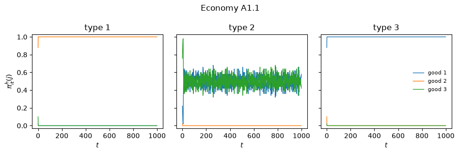
Only type 2 agents carry any randomness, and the reason is instructive: they are the agents who use good 1 as money, so which good they are holding depends on where they are in the cycle “acquire money, spend money”.
Now let us look at the trades themselves.
The entry in row \(i\), column \(j\) is the triple over \(k\) of the frequency with which a type \(i\) agent holds \(j\), meets someone holding \(k\), and trades.
exchanges(sim_a11)
| good 1 | good 2 | good 3 | |
|---|---|---|---|
| type 1 | (0.00, 0.00, 0.00) | (0.15, 0.00, 0.00) | (0.00, 0.00, 0.00) |
| type 2 | (0.09, 0.15, 0.00) | (0.00, 0.00, 0.00) | (0.16, 0.00, 0.00) |
| type 3 | (0.00, 0.00, 0.16) | (0.00, 0.00, 0.00) | (0.00, 0.00, 0.00) |
The exchange pattern is easier to read as a picture.
plot_flows(sim_a11, title="Economy A1.1: discovered exchange pattern")
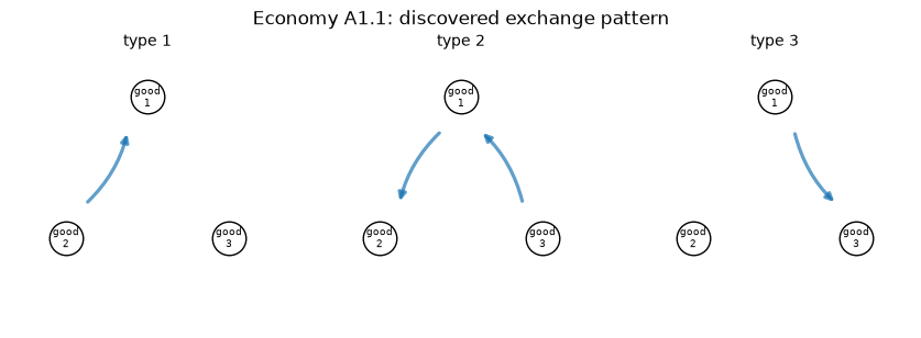
This is exactly the fundamental equilibrium triangle: type 1 gives up good 2 for good 1, type 3 gives up good 1 for good 3, and type 2 runs both legs, giving up good 3 for good 1 and later good 1 for good 2.
Good 1 circulates as money.
We can also ask what the winning rules would do in states that are never visited, which is what Kiyotaki and Wright’s strategies specify and what the paper reports.
winning_actions(sim_a11)
| good 1 | good 2 | good 3 | |
|---|---|---|---|
| type 1 | (0,0,0) | (1,0,0) | (1,0,0) |
| type 2 | (1,1,0) | (0,0,0) | (1,1,0) |
| type 3 | (0,0,1) | (0,0,0) | (0,0,0) |
Reading row “type 1”, the entry in column “good 2” is the triple \((\tilde\pi^e_1(21|2), \tilde\pi^e_1(22|2), \tilde\pi^e_1(23|2))\).
A type 1 agent holding good 2 accepts good 1 and refuses good 3: he does not speculate.
Finally, we can look inside a classifier system and read off the rules that won the competition.
strongest(sim_a11.agents[0].trade)
| classifier | strength | times used | |
|---|---|---|---|
| 0 | 0110 -> 1 | 30.04 | 8343 |
| 1 | 1010 -> 0 | 29.27 | 5 |
| 2 | 1001 -> 0 | 27.54 | 8 |
| 3 | 1000 -> 0 | 16.80 | 3 |
| 4 | 1001 -> 1 | 0.00 | 1 |
strongest(sim_a11.agents[0].consume)
| classifier | strength | times used | |
|---|---|---|---|
| 0 | 10 -> 1 | 66.20 | 8354 |
| 1 | 10 -> 0 | -0.10 | 2 |
| 2 | 0# -> 1 | -0.55 | 41625 |
| 3 | #0 -> 1 | -0.68 | 6 |
| 4 | 00 -> 1 | -0.75 | 3 |
The strongest exchange rule for a type 1 agent is 0110 -> 1, that is, “if I am holding
good 2 (01) and my partner holds good 1 (10), trade” – and it is used thousands of
times, while the runners-up are essentially never used.
The strongest consumption rule is 10 -> 1: “if I am holding good 1, eat it”.
These are exactly the classifiers \(e^1_{2,1,1}\) and \(c^1_{1,1}\) that the paper shows support the fundamental equilibrium.
89.6. Economy A2.1: when theory predicts speculation#
Economy A2 differs from A1 only in that \(u_i = 500\) instead of \(100\).
That is enough to violate the Kiyotaki-Wright inequality (89.4), so for patient agents the unique stationary rational-expectations equilibrium is now the speculative one, in which type 1 agents accept good 3 in the expectation of trading it for good 1.
Do our adaptive agents find it?
economy_a21 = Economy(
    name='A2.1',
    produces=np.array([1, 2, 0]),
    storage_costs=np.array([0.1, 1.0, 20.0]),
    u=500.0,
    method='enumerate',
)

sim_a21 = Simulation(economy_a21, seed=42)
sim_a21.run(1000)

holdings(sim_a21)
| good 1 | good 2 | good 3 | |
|---|---|---|---|
| type 1 | 0.00 | 1.0 | 0.00 |
| type 2 | 0.53 | 0.0 | 0.47 |
| type 3 | 1.00 | 0.0 | 0.00 |
Here is the speculative equilibrium that Kiyotaki and Wright’s theory predicts for these parameters, for comparison.
speculative = pd.DataFrame([[0, 0.707, 0.293],
                            [0.586, 0, 0.414],
                            [1, 0, 0]],
                           index=type_names(economy_a21),
                           columns=good_names(economy_a21))
speculative
| good 1 | good 2 | good 3 | |
|---|---|---|---|
| type 1 | 0.000 | 0.707 | 0.293 |
| type 2 | 0.586 | 0.000 | 0.414 |
| type 3 | 1.000 | 0.000 | 0.000 |
The answer is no.
The simulated holdings are those of the fundamental equilibrium: type 1 agents hold good 2 essentially always and never accumulate good 3, whereas speculation requires them to hold good 3 nearly thirty percent of the time.
It is worth looking at why.
winning_actions(sim_a21)
| good 1 | good 2 | good 3 | |
|---|---|---|---|
| type 1 | (0,0,0) | (1,0,0) | (0,1,0) |
| type 2 | (1,1,0) | (0,0,0) | (1,1,0) |
| type 3 | (0,0,1) | (0,0,0) | (0,0,0) |
Reading row “type 1”, column “good 2”, the winning exchange rule refuses good 3: type 1 agents will not make the speculative swap.
Now look at what they would do with good 3 if they had it.
consume_actions(sim_a21)
| good 1 | good 2 | good 3 | |
|---|---|---|---|
| type 1 | 1 | 1 | 1 |
| type 2 | 0 | 1 | 0 |
| type 3 | 1 | 1 | 1 |
strongest(sim_a21.agents[0].consume, n=4)
| classifier | strength | times used | |
|---|---|---|---|
| 0 | 10 -> 1 | 333.70 | 8161 |
| 1 | ## -> 1 | 0.17 | 41809 |
| 2 | 10 -> 0 | -0.10 | 2 |
| 3 | #0 -> 1 | -0.66 | 17 |
This is the paper’s diagnosis, visible in the output.
One consumption rule, 10 -> 1, is specific and enormously strong: “if I hold good 1, eat
it”.
The rule that decides everything else is ## -> 1 – eat whatever you are holding – a
maximally general rule with two wildcards and a strength barely above zero, yet it is the
strongest rule matching any state other than “holding good 1”.
So a type 1 agent who acquired good 3 would immediately consume it for zero utility rather than carry it and trade it for good 1.
As the paper puts it, the winning consumption classifiers of type 1 agents are too general – they have too many \(\#\)’s to distinguish among stored goods – so type 1 agents overconsume good 3, and the information that would make speculation pay never reaches the exchange classifiers.
The authors’ diagnosis is worth quoting:
Patience requires experience. The transfer system inside the classifier system is designed to converge to a set of long-run average strengths. In the limit, the artificially intelligent agents should behave as long-run average payoff maximizers… It takes time, however, for optimal rules to achieve the desired strengths. The behavior of our artificially intelligent agents can be very myopic at the beginning… The present algorithm seems defective in that it has too little experimentation to support the speculative equilibrium even in the long simulations we have run.
Early on, before any rule has accumulated a meaningful average, agents behave myopically, and a myopic agent never accepts an expensive good.
By the time strengths have settled, everyone else has already stopped speculating, so speculation no longer pays.
The equilibrium selected is a consequence of the learning dynamics, not of the payoffs alone.
89.7. Economy B.1: a different production pattern#
Economy B changes the production technology – type 1 produces good 3, type 2 produces good 1, type 3 produces good 2 – and compresses storage costs to \(s = (1, 4, 9)\) with \(u_i = 100\).
Both a fundamental and a speculative equilibrium exist.
The paper reports something striking: at \(t = 500\) the economy looks speculative, but by \(t = 1000\) it has moved to the fundamental equilibrium.
economy_b1 = Economy(
    name='B.1',
    produces=np.array([2, 0, 1]),               # type 1 -> good 3, type 2 -> good 1, ...
    storage_costs=np.array([1.0, 4.0, 9.0]),
    u=100.0,
    method='enumerate',
    b_trade=(0.25, 0.25),
)

sim_b1 = Simulation(economy_b1, seed=42)
sim_b1.run(1000)
holdings(sim_b1, t=500)
| good 1 | good 2 | good 3 | |
|---|---|---|---|
| type 1 | 0.00 | 0.274 | 0.726 |
| type 2 | 1.00 | 0.000 | 0.000 |
| type 3 | 0.56 | 0.440 | 0.000 |
holdings(sim_b1)
| good 1 | good 2 | good 3 | |
|---|---|---|---|
| type 1 | 0.000 | 0.324 | 0.676 |
| type 2 | 1.000 | 0.000 | 0.000 |
| type 3 | 0.626 | 0.374 | 0.000 |
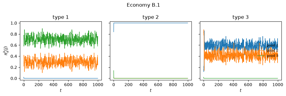
plot_holdings(sim_b1, title="Economy B.1")
paper_b1 = np.array([[0.0, 0.28, 0.72],         # the paper's table at t = 1000
                     [0.994, 0.0, 0.006],
                     [0.526, 0.474, 0.0]])

print(f"max |simulated - paper's table| = "
      f"{np.abs(holdings(sim_b1).to_numpy() - paper_b1).max():.3f}")
max |simulated - paper's table| = 0.100
The end state reproduces the paper’s qualitative pattern, with the largest single discrepancy about a tenth.
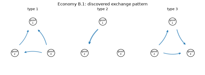
Type 2 agents hold good 1 always, and type 3 agents split their holdings between good 1 and their own production good 2.
The paper reports one further feature that our run does not reproduce.
In the authors’ simulation, type 3 agents held good 2 with probability one at \(t = 500\) – refusing the cheaper good 1, which is the speculative pattern – and only later shifted into good 1:
Economy B.1 displays an interesting pattern of evolution. At iteration 500 the distribution of holdings and, especially, the trading patterns correspond to the speculative equilibrium. However, the economy moves away from this state and by iteration 1000 has practically converged to the fundamental equilibrium.
In our implementation the shift happens within the first fifty periods, so the speculative phase is over before \(t = 500\).
The transient is evidently sensitive to details of the implementation in a way that the limit is not.
The economics of the authors’ observation is nevertheless worth stating, because it bears on how we should read Economy A2.
There, one might suspect that the fundamental equilibrium was selected merely because myopic agents refuse expensive goods from the very beginning.
In Economy B the system starts in the speculative pattern and moves away from it as strengths accumulate, which suggests that the selection of the fundamental equilibrium is something the learning dynamics do, not just an artifact of where they start.
plot_flows(sim_b1, title="Economy B.1: discovered exchange pattern")
89.8. The genetic algorithm#
Complete enumeration is only feasible because the Kiyotaki-Wright state space is tiny.
In any larger problem the list of all conceivable rules is far too long to carry around, and an agent must instead work with a limited population of rules that is continually revised.
Marimon, McGrattan and Sargent add four operations for this case.
Creation and diversification we have already implemented; they handle unforeseen states and guarantee that both actions get tried.
For the five-good economy we shall use a variant of diversification that clones the winning rule with the opposite action, thereby preserving the winner’s level of generality rather than manufacturing a fully specific rule.
def diversify_clone(rules, matches, winner, ufitness=0.5):
    "Copy the winner with the opposite action over a rarely used rule."
    if len(set(rules.action[matches])) > 1:
        return
    losers = np.flatnonzero(rules.used / (rules.used.max() + 1) < ufitness)
    if losers.size == 0:
        return
    j = losers[np.argmin(rules.strength[losers])]
    rules.replace(j, rules.cond[winner].copy(), 1 - rules.action[winner],
                  rules.strength[winner], used=rules.used[winner])
Specialization turns wildcards into specific bits, so that a rule which has been serving several states can split off a sharper version of itself.
It is called with a probability \(f_s(t) = 1/(2\sqrt{t})\) that declines over time: experimentation is cheap early and expensive late.
def specialize_all(rules, t, rng):
    "Replace each wildcard by a bit with probability 1 / (2 sqrt(t))."
    hit = (rules.cond == WILD) & (rng.random(rules.cond.shape)
                                  < 1.0 / (2.0 * np.sqrt(t)))
    if hit.any():
        rules.cond[hit] = rng.integers(0, 2, size=hit.sum())


def specialize_winner(rules, winner, pmutation, rng, ufitness=0.5):
    "Plant a sharpened copy of a heavily used winner over a rarely used rule."
    cond = rules.cond[winner]
    if not np.any(cond == WILD):
        return
    if rules.used[winner] / (rules.used.max() + 1) <= ufitness:
        return
    pick = (cond == WILD) & (rng.random(cond.shape) < pmutation)
    losers = np.flatnonzero(rules.used / (rules.used.max() + 1) < ufitness)
    if not pick.any() or losers.size == 0:
        return
    j = losers[np.argmin(rules.strength[losers])]
    new = cond.copy()
    new[pick] = rng.integers(0, 2, size=pick.sum())
    rules.replace(j, new, rules.action[winner], rules.strength[winner],
                  used=rules.used[winner])
Generalization is the genetic algorithm proper.
Rules that are weak or rarely used become candidates for replacement.
Parents are drawn in two stages – first a subset weighted by how often rules have been used, then a roulette wheel on strength within that subset – so that a rule must be both successful and relevant to reproduce.
Two children are formed by crossover and, in the 'ga3' variant, mutation.
Each child then displaces the rule it most closely resembles among the replaceable ones, a device known as crowding that preserves diversity by making children compete against their own kind.
The 'ga4' variant replaces single-point crossover with a generalizing crossover: inside
a randomly drawn interval, positions where the parents disagree become wildcards.
This is the operator described in section 6 of the paper and illustrated in its figure 5, and it manufactures general rules rather than recombining specific ones.
def roulette(weights, rng):
    total = weights.sum()
    if total <= 0:
        return int(rng.integers(0, len(weights)))
    return int(np.searchsorted(np.cumsum(weights), rng.random() * total))


def crowding_victim(rules, cond, action, cankill, rng, crowd_factor, crowd_subpop):
    "De Jong crowding: the child displaces the replaceable rule it resembles most."
    size = max(1, int(crowd_subpop * len(cankill)))
    best, best_sim = cankill[0], -1
    for _ in range(crowd_factor):
        pool = (cankill if size >= len(cankill)
                else list(rng.choice(cankill, size=size, replace=False)))
        cand = min(pool, key=lambda i: rules.strength[i])
        sim = (np.count_nonzero(cond == rules.cond[cand])
               + (action != rules.action[cand]))
        if sim > best_sim:
            best, best_sim = cand, sim
    return best


def genetic_algorithm(rules, rng, generalize=False, pcross=0.6, pmutation=0.01,
                      propselect=0.2, propused=0.7, crowd_factor=8,
                      crowd_subpop=0.5, uratio=(0.0, 0.2)):
    n, L = rules.n, rules.length
    if n < 4:
        return

    # rules that are weak or seldom used may be replaced
    max_used = max(rules.used.max() + (1 if generalize else 0), 1)
    cankill = list(np.flatnonzero((rules.strength < uratio[0]) |
                                  (rules.used / max_used < uratio[1])))
    if not cankill:
        return

    fitness = rules.strength - min(rules.strength.min(), 0.0) + 1e-6
    n_pairs = min(max(1, round(propselect * n * 0.5)), (len(cankill) + 1) // 2)
    n_called = int(propused * n)

    for _ in range(n_pairs):
        if not cankill:
            break

        # stage 1: pre-select a pool with probability proportional to usage
        if n_called < n:
            avail = rules.used.astype(float) + 1.0
            pool = []
            for _ in range(n_called):
                if avail.sum() <= 0:
                    break
                k = roulette(avail, rng)
                pool.append(k)
                avail[k] = 0.0
            if len(pool) < 2:
                pool = list(range(n))
        else:
            pool = list(range(n))
        pool = np.array(pool)

        # stage 2: roulette wheel on fitness within the pool
        mum, dad = pool[roulette(fitness[pool], rng)], pool[roulette(fitness[pool], rng)]
        kids = [rules.cond[mum].copy(), rules.cond[dad].copy()]
        acts = [rules.action[mum], rules.action[dad]]
        avg = 0.5 * (rules.strength[mum] + rules.strength[dad])

        if generalize:
            # two-point crossover in which disagreements become wildcards
            lo, hi = np.sort(rng.integers(0, L + 1, size=2))
            inside = rng.random() > 0.5
            region = (np.arange(lo, hi) if inside else
                      np.concatenate([np.arange(0, lo), np.arange(hi, L)]))
            for j in region:
                a, b = kids[0][j], kids[1][j]
                if a >= 0 and b >= 0 and a != b:
                    kids[0][j] = kids[1][j] = WILD
        else:
            # single-point crossover with ternary mutation
            jc = 1 + int((L - 1) * rng.random()) if rng.random() < pcross else L
            kids = [np.concatenate([rules.cond[mum][:jc], rules.cond[dad][jc:]]),
                    np.concatenate([rules.cond[dad][:jc], rules.cond[mum][jc:]])]
            for k in range(2):
                flip = rng.random(L) < pmutation
                if flip.any():
                    shift = rng.integers(1, 3, size=flip.sum())
                    kids[k][flip] = ((kids[k][flip] + 1 + shift) % 3) - 1
                if rng.random() < pmutation:
                    acts[k] = 1 - acts[k]

        for k, parent in zip(range(2), (mum, dad)):
            if not cankill:
                break
            j = crowding_victim(rules, kids[k], acts[k], cankill, rng,
                                crowd_factor, crowd_subpop)
            rules.replace(j, kids[k], acts[k], avg,
                          used=rules.used[parent], traded=rules.traded[parent])
            cankill.remove(j)
89.9. Economy A1.2: learning from random rules#
Economy A1.2 has the same parameters as A1.1, but agents now begin with 72 exchange rules and 12 consumption rules drawn at random.
Most of these rules are nonsense, and there is no guarantee that the population even contains the rules needed to support an equilibrium.
The genetic operators must manufacture them.
economy_a12 = Economy(
    name='A1.2',
    produces=np.array([1, 2, 0]),
    storage_costs=np.array([0.1, 1.0, 20.0]),
    u=100.0,
    method='ga3',
)

sim_a12 = Simulation(economy_a12, seed=2)
sim_a12.run(2000, verbose=True)
  period   200:  trades =  33,  consumptions =  14
  period   400:  trades =   4,  consumptions =   0
  period   600:  trades =  37,  consumptions =  18
  period   800:  trades =  44,  consumptions =   0
  period  1000:  trades =  30,  consumptions =  15
  period  1200:  trades =  32,  consumptions =  17
  period  1400:  trades =  31,  consumptions =  14
  period  1600:  trades =  48,  consumptions =  17
  period  1800:  trades =  40,  consumptions =  41
  period  2000:  trades =  63,  consumptions =  41
holdings(sim_a12, t=1000)
| good 1 | good 2 | good 3 | |
|---|---|---|---|
| type 1 | 0.0 | 1.0 | 0.0 |
| type 2 | 0.0 | 0.0 | 1.0 |
| type 3 | 1.0 | 0.0 | 0.0 |
holdings(sim_a12)
| good 1 | good 2 | good 3 | |
|---|---|---|---|
| type 1 | 0.000 | 1.0 | 0.000 |
| type 2 | 0.478 | 0.0 | 0.522 |
| type 3 | 1.000 | 0.0 | 0.000 |
plot_holdings(sim_a12, title="Economy A1.2")
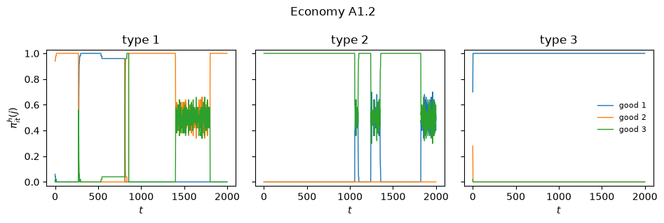
The fundamental equilibrium is reached again, though it takes noticeably longer and the early transition is much less orderly than under complete enumeration.
Let us see which rules survived.
strongest(sim_a12.agents[0].trade, n=6)
| classifier | strength | times used | |
|---|---|---|---|
| 0 | 0110 -> 1 | 30.20 | 15642 |
| 1 | 1010 -> 1 | 28.19 | 32 |
| 2 | 0010 -> 1 | 27.74 | 7933 |
| 3 | 1010 -> 1 | 27.41 | 32 |
| 4 | 0110 -> 1 | 27.41 | 6422 |
| 5 | 1010 -> 1 | 27.05 | 32 |
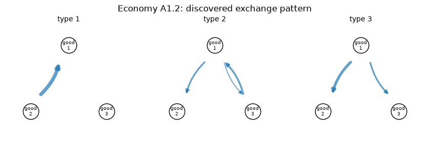
The population has converged onto near-copies of a single rule.
0110 -> 1 – “holding good 2, meeting good 1, trade” – is exactly the rule that complete
enumeration selected in Economy A1.1, but here the genetic algorithm had to build it, and
several copies of it now occupy the population.
The other entries are its offspring: 0111 -> 1 has the same own-holding condition but a
partner condition of 11, which is not the code of any of the three goods, so that rule can
never fire.
It carries a high strength and a large usage count only because children inherit both from their parents.
plot_flows(sim_a12, title="Economy A1.2: discovered exchange pattern")
Warning
Convergence is not guaranteed run by run.
With random initial rules the population sometimes fails to manufacture the rules needed for the fundamental equilibrium within 2000 periods, and the economy settles into a pattern with little trade.
Try changing the seed above to see this.
The paper is explicit that the algorithm has “too little experimentation” and that improving it is unfinished business.
89.10. Economy C: fiat money#
Now add a fourth object, good 0, which
costs nothing to store, \(s_0 = 0\);
yields no utility to anybody; and
cannot be consumed.
It is intrinsically worthless.
It is introduced by handing 48 units of it to 48 randomly chosen agents at \(t = 0\), and commodity storage costs are raised to \(s = (9, 14, 29)\) so that no commodity is nearly as cheap to store as money.
If a good like this circulates, it can only be because agents have discovered that other agents will take it.
economy_c = Economy(
    name='C',
    produces=np.array([1, 2, 0]),
    storage_costs=np.array([9.0, 14.0, 29.0, 0.0]),    # last good is fiat money
    u=100.0,
    method='ga3',
    n_trade_rules=150,
    n_consume_rules=20,
    b_consume=(0.025, 0.25),
    n_fiat=48,
    start='production',
)

sim_c = Simulation(economy_c, seed=2)
sim_c.run(2000, verbose=True)
  period   200:  trades =  53,  consumptions =  32
  period   400:  trades =  35,  consumptions =  29
  period   600:  trades =  61,  consumptions =  40
  period   800:  trades =  53,  consumptions =  26
  period  1000:  trades =  50,  consumptions =  37
  period  1200:  trades =  49,  consumptions =  32
  period  1400:  trades =  45,  consumptions =  23
  period  1600:  trades =  55,  consumptions =  38
  period  1800:  trades =  63,  consumptions =  36
  period  2000:  trades =  52,  consumptions =  26
holdings(sim_c, t=750)
| good 1 | good 2 | good 3 | fiat | |
|---|---|---|---|---|
| type 1 | 0.000 | 0.514 | 0.212 | 0.274 |
| type 2 | 0.228 | 0.000 | 0.318 | 0.454 |
| type 3 | 0.768 | 0.000 | 0.000 | 0.232 |
holdings(sim_c, t=1250)
| good 1 | good 2 | good 3 | fiat | |
|---|---|---|---|---|
| type 1 | 0.000 | 0.782 | 0.000 | 0.218 |
| type 2 | 0.242 | 0.000 | 0.388 | 0.370 |
| type 3 | 0.628 | 0.000 | 0.000 | 0.372 |
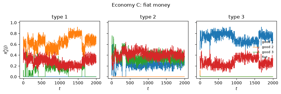
Compare with the paper’s table at \(t = 1250\), where the columns are (good 1, good 2, good 3, fiat): \((0, 0.54, 0, 0.46)\) for type 1, \((0.18, 0, 0.53, 0.28)\) for type 2, and \((0.77, 0, 0, 0.21)\) for type 3.
Every type holds fiat money a substantial fraction of the time.
plot_holdings(sim_c, title="Economy C: fiat money")
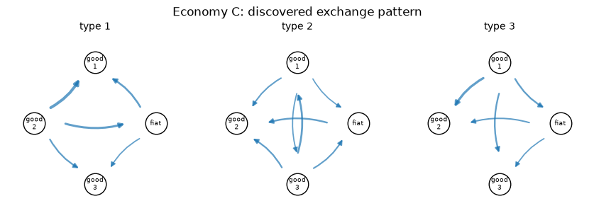
plot_flows(sim_c, title="Economy C: discovered exchange pattern")
winning_actions(sim_c)
| good 1 | good 2 | good 3 | fiat | |
|---|---|---|---|---|
| type 1 | (1,-,-,-) | (1,1,1,1) | (1,-,-,-) | (1,0,1,1) |
| type 2 | (1,1,1,1) | (-,1,-,1) | (1,1,1,1) | (0,1,0,1) |
| type 3 | (1,1,1,1) | (-,-,1,-) | (-,-,1,-) | (0,1,1,1) |
The arrows into and out of the fiat node show money changing hands in both directions for every type: agents give up commodities to acquire it and give it up to acquire the commodity they consume.
Nothing in the environment told them to do this.
Each agent discovered only that rules which end up holding the costless object earn more than rules that do not – and, because everyone was discovering this at once, the belief became self-confirming.
This is a genuinely social arrangement built by agents who individually understand nothing about it.
89.11. Economy D: five goods, five types#
The last economy has five types and five goods, with production
type \(i\) |
produces |
consumes |
|---|---|---|
1 |
good 3 |
good 1 |
2 |
good 4 |
good 2 |
3 |
good 5 |
good 3 |
4 |
good 1 |
good 4 |
5 |
good 2 |
good 5 |
storage costs \(s = (1, 4, 9, 16, 30)\) and \(u_i = 200\).
Goods are now encoded in three bits, and each agent carries 180 exchange rules and 20 consumption rules – a small fraction of the possible rules, so the genetic algorithm is essential.
The authors emphasize that they had no analytical characterization of equilibrium for this economy before running it.
The simulation is being used as a device to discover what an equilibrium might look like, which could then be verified analytically.
economy_d = Economy(
    name='D',
    produces=np.array([2, 3, 4, 0, 1]),         # type 1 -> good 3, type 2 -> good 4, ...
    storage_costs=np.array([1.0, 4.0, 9.0, 16.0, 30.0]),
    u=200.0,
    method='ga4',
    n_trade_rules=180,
    n_consume_rules=20,
    start='production',
)

sim_d = Simulation(economy_d, seed=3)
sim_d.run(2000, verbose=True)
  period   200:  trades =  41,  consumptions =  21
  period   400:  trades =  65,  consumptions =  26
  period   600:  trades =  38,  consumptions =  22
  period   800:  trades =  28,  consumptions =  20
  period  1000:  trades =  36,  consumptions =  26
  period  1200:  trades =  42,  consumptions =  13
  period  1400:  trades =  34,  consumptions =   5
  period  1600:  trades =  36,  consumptions =  25
  period  1800:  trades =  34,  consumptions =  19
  period  2000:  trades =  40,  consumptions =  23
holdings(sim_d, t=500)
| good 1 | good 2 | good 3 | good 4 | good 5 | |
|---|---|---|---|---|---|
| type 1 | 0.000 | 0.000 | 0.972 | 0.012 | 0.016 |
| type 2 | 0.274 | 0.000 | 0.504 | 0.212 | 0.010 |
| type 3 | 0.000 | 0.000 | 0.000 | 0.000 | 1.000 |
| type 4 | 0.994 | 0.000 | 0.006 | 0.000 | 0.000 |
| type 5 | 0.972 | 0.024 | 0.000 | 0.004 | 0.000 |
holdings(sim_d)
| good 1 | good 2 | good 3 | good 4 | good 5 | |
|---|---|---|---|---|---|
| type 1 | 0.0 | 0.588 | 0.324 | 0.008 | 0.080 |
| type 2 | 0.0 | 0.000 | 0.062 | 0.926 | 0.012 |
| type 3 | 0.0 | 0.170 | 0.000 | 0.074 | 0.756 |
| type 4 | 1.0 | 0.000 | 0.000 | 0.000 | 0.000 |
| type 5 | 0.0 | 0.952 | 0.046 | 0.002 | 0.000 |
plot_holdings(sim_d, title="Economy D: five goods, five types")
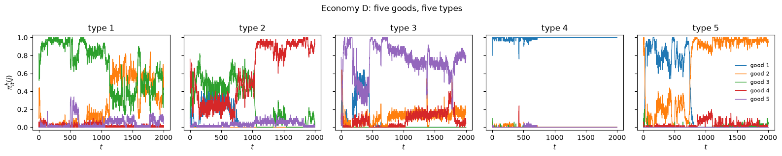
Two features stand out.
First, the diagonal is zero: no type ever ends a period holding the good it consumes, because it consumes it.
Second, each type accumulates its own production good together with goods that are cheaper to store, never more expensive.
Type 3, for instance, produces good 5, the most expensive good in the economy, and holds it only part of the time, having traded some of it away for the much cheaper good 2.
Type 4 produces good 1, the cheapest good of all, and simply holds it.
Let us classify the trades that actually take place.
def trade_composition(sim, window=200):
    """
    Classify realized trades by what the agent acquires: its own consumption
    good, a good that is cheaper to store than the one given up, or neither.
    """
    econ = sim.econ
    f = np.array(sim.exch_hist)[-window:].sum(axis=0)
    s = econ.storage_costs
    counts = {'own consumption good': 0.0, 'a cheaper good': 0.0, 'neither': 0.0}
    for i in range(econ.n_types):
        for j in range(econ.n_goods):
            for k in range(econ.n_goods):
                if j == k:
                    continue
                key = ('own consumption good' if k == i else
                       'a cheaper good' if s[k] < s[j] else 'neither')
                counts[key] += f[i, j, k]
    total = sum(counts.values())
    return pd.Series({k: round(v / total, 3) for k, v in counts.items()},
                     name='share of realized trades')


trade_composition(sim_d)
own consumption good    0.364
a cheaper good          0.301
neither                 0.335
Name: share of realized trades, dtype: float64
Roughly two thirds of realized trades acquire either the agent’s own consumption good or a good that is cheaper to store, which is the pattern the paper describes.
The remaining third deserves a comment, because it is not evidence against that pattern.
Consider a type 1 agent, who produces good 3, swapping good 3 for the far more expensive good 5.
He then consumes good 5 – getting no utility from it – and produces good 3 again, so he ends the period holding good 3 and paying \(s_3\), exactly as he would have had he refused.
Such trades are payoff-neutral, so nothing in the accounting system pushes the rules that generate them out of the population.
plot_flows(sim_d, window=200, cutoff=0.03,
           title="Economy D: discovered exchange pattern")
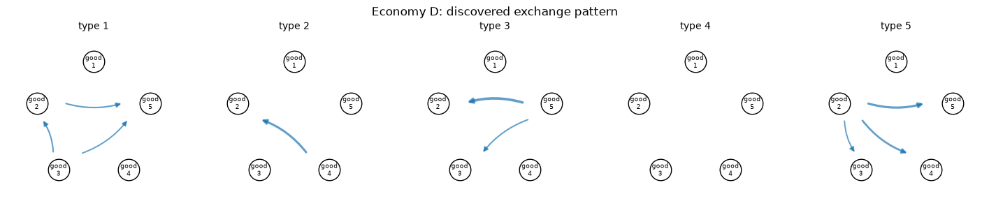
The paper summarizes what it sees in these patterns:
From the simulation results, we can see that the trading patterns nearly seem to describe a fundamental equilibrium in which agents are only willing to trade for commodities of lower cost than the one currently in storage, except that they always accept the commodity of their type. Some speculative moves can be detected.
An example of such a speculative move is a type 2 agent accepting good 3 for good 1, not because good 3 is cheap but because type 3 agents will take it in exchange for good 2.
89.12. Concluding remarks#
Marimon, McGrattan and Sargent’s agents know very little.
They do not know their own utility functions, they do not know storage costs, they do not know the distribution of goods across the population, and they certainly do not solve dynamic programs.
They recognize utility when they experience it and costs when they bear them, and they keep running averages.
Out of this the following emerges:
Nash-Markov behavior is learnable. In most of the economies simulated, holdings and trading patterns converge to a stationary Nash equilibrium of the Kiyotaki-Wright model.
Learning selects among equilibria. Where the rational-expectations model admits both a fundamental and a speculative equilibrium, the classifier systems always found the fundamental one.
Economy A2 shows they found it even where theory says it should not be an equilibrium at all for patient agents.
Economy B shows this is not simply early myopia, since that economy moves away from a speculative pattern as it learns.
Institutions can be discovered. Economy C’s agents built a fiat monetary system out of nothing but their own experience of storage costs.
The method scales. Economy D produced a credible description of equilibrium in a model its authors had not solved.
The paper is candid about what is missing.
There are no convergence theorems, only a sketch of how stochastic approximation arguments might supply them; and the authors judge their genetic algorithm to provide “too little experimentation” – which is precisely why the speculative equilibrium never appears.
That diagnosis, that an adaptive system’s selection among equilibria is governed by how much it explores and when, has proved durable.
89.13. Exercises#
Exercise 89.1
Economy A2.2 is Economy A2 – with \(u_i = 500\) – but started from randomly generated rules
and evolved with the 'ga3' genetic algorithm, exactly as A1.2 relates to A1.1.
The paper’s summary table lists its equilibrium type as speculative, and the authors report that after 1000 iterations the economy had not converged, with trading patterns closer to the fundamental equilibrium at \(t = 1000\) than at \(t = 500\).
Simulate it for 2000 periods and report holdings at \(t = 500\), \(t = 1000\) and \(t = 2000\).
Does the extra experimentation supplied by the genetic algorithm produce speculation?
Solution
economy_a22 = Economy(
    name='A2.2',
    produces=np.array([1, 2, 0]),
    storage_costs=np.array([0.1, 1.0, 20.0]),
    u=500.0,
    method='ga3',
)

sim_a22 = Simulation(economy_a22, seed=3)
sim_a22.run(2000)

for t in (500, 1000, 2000):
    print(f"\nt = {t}")
    print(holdings(sim_a22, t=t))
t = 500
        good 1  good 2  good 3
type 1    0.00     1.0    0.00
type 2    0.47     0.0    0.53
type 3    1.00     0.0    0.00

t = 1000
        good 1  good 2  good 3
type 1   0.000     1.0   0.000
type 2   0.492     0.0   0.508
type 3   1.000     0.0   0.000

t = 2000
        good 1  good 2  good 3
type 1   0.000     1.0   0.000
type 2   0.494     0.0   0.506
type 3   1.000     0.0   0.000
plot_holdings(sim_a22, title="Economy A2.2")
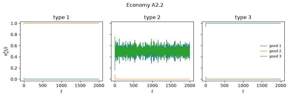
The economy again settles on the fundamental pattern: type 1 holds good 2, type 3 holds good 1, and type 2 alternates between goods 1 and 3.
Type 1 agents are not holding good 3, so they are not speculating.
Randomizing the initial rules and letting the genetic algorithm run does not by itself generate enough experimentation to sustain speculation – which is the paper’s own conclusion.
Exercise 89.2
Economy B.2 is Economy B started from random rules with the 'ga3' genetic algorithm.
The paper reports that it “had not converged after 2000 periods” but was “moving towards the fundamental equilibrium”, with holdings at \(t = 2000\) of \((0, 0.354, 0.646)\) for type 1, \((0.996, 0, 0.004)\) for type 2 and \((0.268, 0.732, 0)\) for type 3.
Simulate it and compare with the complete-enumeration Economy B.1 that we ran above.
Solution
economy_b2 = Economy(
    name='B.2',
    produces=np.array([2, 0, 1]),
    storage_costs=np.array([1.0, 4.0, 9.0]),
    u=100.0,
    method='ga3',
)

sim_b2 = Simulation(economy_b2, seed=1)
sim_b2.run(2000)

for t in (500, 1000, 2000):
    print(f"B.2 at t = {t}")
    print(holdings(sim_b2, t=t))
    print()
print("B.1 (complete enumeration) at t = 1000, for comparison")
print(holdings(sim_b1))
B.2 at t = 500
        good 1  good 2  good 3
type 1   0.000   0.304   0.696
type 2   0.676   0.000   0.324
type 3   0.336   0.664   0.000

B.2 at t = 1000
        good 1  good 2  good 3
type 1   0.000   0.252   0.748
type 2   1.000   0.000   0.000
type 3   0.506   0.494   0.000

B.2 at t = 2000
        good 1  good 2  good 3
type 1   0.000   0.262   0.738
type 2   1.000   0.000   0.000
type 3   0.472   0.528   0.000

B.1 (complete enumeration) at t = 1000, for comparison
        good 1  good 2  good 3
type 1   0.000   0.324   0.676
type 2   1.000   0.000   0.000
type 3   0.626   0.374   0.000
plot_holdings(sim_b2, title="Economy B.2")
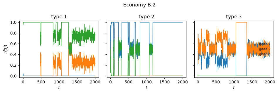
Follow the two types that move.
Type 2 agents are still split at \(t = 500\) and have locked onto good 1 by \(t = 1000\).
Type 3 agents start out mostly holding their own production good 2 and shift a substantial part of their holdings into the cheaper good 1 over the same interval, which is the movement toward the fundamental equilibrium that the paper describes.
After that the type 3 split stops moving in one direction and rattles around a half-and-half mix from one reading to the next, so this economy has not converged in the sense that B.1 has.
That is the paper’s own verdict on it.
Compared with the complete-enumeration run, the genetic algorithm gets type 1 and type 2 to much the same place and leaves type 3 less far along.
Building the needed rules from random material costs time that the enumerated economy never had to spend.
Exercise 89.3
The bid functions \(b_1(e) = b_{11} + b_{12}\sigma_e\) favor specific rules over general ones, since \(\sigma_e\) falls with the number of wildcards.
What happens if this tilt is removed?
Rerun Economy A1.1 with \(b_{12} = 0\), holding \(b_{11} + b_{12}\) fixed at \(0.05\), and compare the number of wildcards in the winning rules with those in the baseline.
A single run will not settle the question, so average over several seeds.
Solution
economy_flat = Economy(
    name='A1.1 with no specificity premium',
    produces=np.array([1, 2, 0]),
    storage_costs=np.array([0.1, 1.0, 20.0]),
    u=100.0,
    method='enumerate',
    b_trade=(0.05, 0.0),
)

sim_flat = Simulation(economy_flat, seed=42)
sim_flat.run(1000)

print(holdings(sim_flat))
        good 1  good 2  good 3
type 1    0.00     1.0    0.00
type 2    0.53     0.0    0.47
type 3    1.00     0.0    0.00
The holdings are unchanged: the fundamental equilibrium is reached either way.
What changes is the kind of rule that gets there.
def wildcards_in_winners(sim):
    "Average number of wildcards in the exchange rule that wins in each state."
    econ = sim.econ
    counts = []
    for A in sim.agents:
        for j in range(econ.n_goods):
            for k in range(econ.n_goods):
                w, _ = auction(A.trade, np.concatenate([econ.code(j), econ.code(k)]))
                if w >= 0:
                    counts.append(np.count_nonzero(A.trade.cond[w] == WILD))
    return np.mean(counts)


def average_wildcards(b_trade, seeds=range(8)):
    out = []
    for seed in seeds:
        econ = Economy(name='sweep', produces=np.array([1, 2, 0]),
                       storage_costs=np.array([0.1, 1.0, 20.0]), u=100.0,
                       method='enumerate', b_trade=b_trade)
        sim = Simulation(econ, seed=seed)
        sim.run(1000)
        out.append(wildcards_in_winners(sim))
    return np.array(out)


base = average_wildcards((0.025, 0.025))
flat = average_wildcards((0.05, 0.0))

pd.DataFrame({"baseline $b_{12} = 0.025$": base.round(2),
              "no premium $b_{12} = 0$": flat.round(2)},
             index=pd.Index(range(8), name="seed"))
| baseline $b_{12} = 0.025$ | no premium $b_{12} = 0$ | |
|---|---|---|
| seed | ||
| 0 | 0.30 | 0.19 |
| 1 | 0.00 | 0.00 |
| 2 | 0.19 | 0.30 |
| 3 | 0.33 | 0.33 |
| 4 | 0.22 | 0.41 |
| 5 | 0.07 | 0.22 |
| 6 | 0.07 | 0.11 |
| 7 | 0.22 | 0.37 |
print(f"mean wildcards, baseline           : {base.mean():.3f}")
print(f"mean wildcards, no specificity bid : {flat.mean():.3f}")
print(f"higher without the premium in {np.sum(flat > base)} of {len(base)} seeds")
mean wildcards, baseline           : 0.176
mean wildcards, no specificity bid : 0.241
higher without the premium in 5 of 8 seeds
Removing the specificity premium raises the average generality of the winning rules, but the effect is modest and does not show up in every run.
That is worth knowing rather than glossing over.
With a complete enumeration the specific rules are all present from the start and accumulate strength on their own, so the bid premium is only one of the forces tilting the auction toward them; the counter is a genuine tendency visible in the average rather than a law obeyed run by run.
The tilt matters more where it is harder to see.
It is the mechanism the paper blames for the failure of Economy A2: general consumption classifiers cannot tell stored goods apart, so they cannot transmit to the exchange classifiers the information that would make speculation profitable.