93. Credible Government Policies#
93.1. Overview#
The Credibility Problem left the government in a trap.
Without a technology for committing itself, a government that re-optimizes every period ends at the Nash outcome, inflating at rate \(\theta U^*\) and getting nothing for it.
That was a one-period story, and it invited an obvious objection: a government that expects to face the same public again tomorrow has a reputation to protect.
This lecture, following chapter 4 of [Sargent, 1999], takes the objection seriously.
We repeat the Kydland–Prescott economy forever, let the government’s current action depend on the whole history of outcomes, and ask which outcome paths can be supported as subgame perfect equilibria.
The answer is not the one the objection anticipated.
Reputation does not rescue the Ramsey outcome, and it does not confirm the Nash outcome either.
It delivers a continuum of equilibrium values, some better than Nash and some considerably worse, with no principle inside the model to select among them.
That is the conclusion this lecture exists to establish, and Sargent states it in one sentence:
My conclusion is that the multiplicity of credible plans replaces pessimism with agnosticism.
It matters for the argument of the whole suite.
The Rise and Fall of U.S. Inflation rests part of its case against the triumph of natural-rate theory on exactly this weakness: a theory with so many equilibria makes few predictions, so a story that depends on policy makers having learned the right one is doing work the theory cannot do for it.
93.1.1. What we build#
The machinery is the recursive method of Abreu, Pearce, and Stacchetti [Abreu, 1988, Abreu et al., 1990], which computes not an optimal value but the whole set of equilibrium values.
Ordinary dynamic programming iterates an operator that maps continuation values into values.
APS iterate an operator that maps sets of continuation values into sets of values, and the set of subgame perfect equilibrium values is its largest fixed point.
Note
Making a promised value into a state variable, and then doing dynamic programming in that state, is the technique sometimes called dynamic programming squared.
It is the organizing idea of the QuantEcon lectures on Stackelberg plans and of the recursive treatments of Ramsey problems in [Ljungqvist and Sargent, 2018].
This lecture is a compact instance: the state is a promised value, and the object we compute is a set.
We then use the machinery three ways.
We construct particular equilibria by guess-and-verify — infinite repetition of Nash, infinite repetition of something better, and Abreu’s stick-and-carrot, which is worse than Nash.
We compute the best and worst equilibrium values from two small programming problems, and check them against a direct iteration of the APS operator.
And we exhibit three quite different equilibria that all attain the same worst value, which is the sharpest illustration of how little the equilibrium concept pins down.
Note
Sargent’s own advice to the reader is worth passing on: this chapter is difficult if you have not seen the theory before, and a reader willing to accept its verdict — that the theory of credible policy yields agnosticism rather than a prediction — can go straight to Adaptive Expectations and the Phelps Problem without losing the thread of the argument.
Let’s start with our imports:
import matplotlib.pyplot as plt
import numpy as np
from typing import NamedTuple
93.2. The repeated economy#
The one-period economy is the one from The Credibility Problem.
Let \((U, y, x)\) be unemployment, inflation, and the public’s expectation of inflation.
Unemployment obeys the expectations-augmented Phillips curve \(U = U^* - \theta(y - x)\), and the government’s one-period payoff, written as a function of \((x, y)\), is
The government’s one-period best response to an expectation \(x\) is
the Nash outcome is \(y^N = \theta U^*\), and the Ramsey outcome is \(y^R = 0\).
Two things are new.
First, the economy repeats for \(t = 1, 2, \ldots\), and the government ranks outcome paths \((x, y) = \{x_t, y_t\}_{t=1}^\infty\) by
The factor \((1-\delta)\) puts \(V^g\) in the same units as a one-period payoff, so values and one-period returns can be compared directly.
Second, inflation is confined to a bounded interval \(Y = [0, y^\#]\).
The lower bound is the Ramsey outcome; the upper bound \(y^\#\) is what makes the government’s problem non-trivial, as we shall see when we look for the worst equilibrium.
class Model(NamedTuple):
    θ: float = 1.25          # slope of the Phillips curve
    U_star: float = 5.5      # natural rate of unemployment
    y_max: float = 10.0      # y^#, the highest admissible inflation rate
    δ: float = 0.95          # discount factor


def r(m, x, y):
    "One-period government payoff when the public expects x and inflation is y."
    U = m.U_star - m.θ * (y - x)
    return -0.5 * (U**2 + y**2)


def B(m, x):
    "The government's one-period best response to expected inflation x."
    return m.θ * (m.U_star + m.θ * x) / (m.θ**2 + 1)


def y_nash(m):
    return m.θ * m.U_star
Two payoff schedules do all the work below, both read as functions of a single inflation rate \(y\) that the public has come to expect.
The first is the rational-expectations payoff \(r(y, y)\): what the government gets if it delivers the inflation the public expects.
The second is the deviation payoff \(r(y, B(y))\): what it gets if the public expects \(y\) but the government yields to temptation and best-responds.
Both have closed forms worth recording, because they explain everything that follows:
def r_keep(m, y):
    "Payoff from delivering the expected inflation rate: r(y, y)."
    return -0.5 * (m.U_star**2 + y**2)


def r_cheat(m, y):
    "Payoff from best-responding to an expectation of y: r(y, B(y))."
    return -(m.U_star + m.θ * y)**2 / (2 * (1 + m.θ**2))


m = Model()
ys = np.linspace(0, m.y_max, 7)
print("closed forms agree with the definitions:",
      np.allclose(r_keep(m, ys), r(m, ys, ys)),
      np.allclose(r_cheat(m, ys), r(m, ys, B(m, ys))))
closed forms agree with the definitions: True True
Both schedules fall as \(y\) rises, but at different rates, and they cross exactly at the Nash rate, where the temptation to deviate vanishes because \(B(y^N) = y^N\).
grid = np.linspace(0, m.y_max, 400)
yN = y_nash(m)
v_R, v_N = r_keep(m, 0.0), r_keep(m, yN)
v_lo = r_cheat(m, m.y_max)

fig, ax = plt.subplots(figsize=(7.5, 5.5))
ax.plot(grid, r_keep(m, grid), 'C0', lw=1.6, label='$r(y, y)$: deliver what is expected')
ax.plot(grid, r_cheat(m, grid), 'C1', lw=1.6, label='$r(y, B(y))$: deviate')
ax.plot(0.0, v_R, 'ko', ms=6)
ax.annotate('$v^R$', (0.0, v_R), textcoords='offset points', xytext=(8, 4))
ax.plot(yN, v_N, 'ko', ms=6)
ax.annotate('$v^N$', (yN, v_N), textcoords='offset points', xytext=(8, 4))
ax.plot(m.y_max, v_lo, 'ko', ms=6)
ax.annotate('$v_{min}$', (m.y_max, v_lo), textcoords='offset points',
            xytext=(-34, 4))
ax.axvline(yN, color='k', lw=0.6, ls=':')
ax.set_xlabel('inflation rate $y$ expected by the public')
ax.set_ylabel('one-period payoff')
ax.set_title('Figure 4.1: the two payoff schedules and the worst equilibrium value')
ax.legend(loc='lower left')
plt.show()
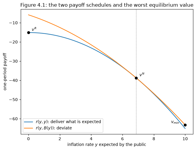
Fig. 93.1 The two payoff schedules: delivering expected inflation against deviating from it#
The vertical gap between the curves is the government’s one-period temptation to inflate less than expected.
It is zero at \(y^N\), and it widens as expected inflation rises above the Nash rate — which is why the worst equilibrium will turn out to live at the top of \(Y\).
93.3. Recursive strategies and promised values#
A government strategy must be able to condition today’s action on the entire past.
Carrying whole histories around is unmanageable, so we follow [Sargent, 1999] in restricting attention to strategies with a recursive representation — a restriction that costs nothing, since it excludes no equilibrium values.
Definition 93.1 (Recursive government strategy)
A recursive government strategy is a pair of functions \(\sigma = (\sigma_1, \sigma_2)\) together with an initial condition \(v_1\), with the structure
where \(v_t\) is a state variable that summarizes the history of outcomes before \(t\).
Each member of the private sector knows \(v_t\) and knows \(\sigma\), and so forecasts
Equation (93.5) builds rational expectations into the private sector: the public is never surprised along the equilibrium path.
A strategy \((\sigma, v_1)\) generates an entire outcome path, and hence a value \(V^g(\sigma, v_1)\) through (93.3).
The theory of credible policy now does something that at first looks like a trick.
It ties the past to the future by requiring the state variable to be the value it generates,
So \(v\) works two shifts at once.
In \(v_{t+1} = \sigma_2(v_t, x_t, y_t)\) it is a bookkeeping device that records what has happened.
In (93.6) it is a promised value — the discounted future the government is owed on entering the period.
Reading it the second way is what makes the machinery go: the strategy hands the government current and future outcomes that make it want to do what is expected of it.
Note
Two readings of \(\sigma\) are available and, within an equilibrium, impossible to tell apart.
It can be a decision rule that the government chooses, or a description of a system of public expectations to which the government conforms.
We return to this ambiguity in the interpretation section, because it is where the theory’s agnosticism comes from.
93.3.1. Historical antecedents#
Formalizing credibility was an achievement of the 1980s, but a sophisticated grasp of the idea is much older.
In 1784 the finance minister Jacques Necker explained to Louis XVI why an absolute monarch, free to renege on debt payments, found it hard to borrow [Sargent and Velde, 1995]:
Therefore one can rekindle or sustain public trust only by giving reassurances on the sovereign’s intentions, and by proving that no motive can incite him to fail his obligations.
Every clause of that sentence is in the modern definition.
A king proves he will never fail his obligations by never wanting to fail them — by conforming to a system of expectations that carries its own incentive constraints, so that at every date and in every contingency his current payoff plus continuation value is higher if he confirms expectations than if he disappoints them.
Definition 93.2 (Subgame perfect equilibrium)
A recursive strategy with promised value \(v\) is a subgame perfect equilibrium (SPE) if and only if
(a) \(\sigma_2(v, \sigma_1(v), \eta)\) is itself a value attainable by a subgame perfect equilibrium, for every \(\eta \in Y\); and
(b) writing \(y = \sigma_1(v)\),
The definition attaches four objects to an equilibrium: a promised value \(v\); a first-period outcome \((y, y)\); a continuation value \(v'\) if the prescribed outcome is observed; and another continuation value \(\tilde v\) if it is not.
In those terms condition (b) reads
which simply says the government does better adhering than departing.
Condition (a) says the continuation values must themselves be equilibrium values.
The definition is circular — equilibrium values appear on both sides — and that circularity is exactly what recursivity buys, and what APS learned to exploit.
93.4. The Abreu–Pearce–Stacchetti method#
Dynamic programming computes an optimal value function by iterating the Bellman equation, a map that turns tomorrow’s value function into today’s.
APS adapted the idea to equilibrium sets.
Start with a candidate set \(W \subset \mathbb{R}\) of continuation values.
Pick a first-period rational-expectations outcome \((y, y)\) and two continuation values from \(W\): a \(w_1\) to reward adherence and a \(w_2\) to punish deviation.
If \(w_1\) is high enough and \(w_2\) low enough, the pair supports \(y\), and delivers the value
Definition 93.3 (Admissibility)
A pair \((y, w)\) is admissible with respect to a set of continuation values \(W\) if there exist \(w_1, w_2 \in W\) with \(w = (1-\delta) r(y,y) + \delta w_1 \geq (1-\delta) r(y,\eta) + \delta w_2\) for all \(\eta \in Y\).
Let \(B(W)\) collect the \(w\) components of all admissible pairs.
This construction builds in condition (b) of Definition 93.2 but ignores condition (a), because the continuation values were drawn from an arbitrary set.
Definition 93.4 (Self-generation)
A set \(W\) of prospective continuation values is self-generating if \(W \subseteq B(W)\).
Every value in a self-generating set is supported by continuation values drawn from that same set — which is condition (a).
APS proved that the set \(V\) of SPE values is the largest self-generating set, that \(B\) maps compact sets into compact sets, that \(B\) is monotone (\(W_2 \subseteq W_1\) implies \(B(W_2) \subseteq B(W_1)\)), and that starting from any \(W_0\) with \(B(W_0) \subseteq W_0\) the iteration \(W_j = B(W_{j-1})\) converges monotonically to \(V = B(V)\).
93.4.1. Computing the operator#
Two simplifications make \(B\) easy to evaluate here.
Because the government’s temptation is worst when it best-responds, the constraint in Definition 93.3 binds hardest at \(\eta = B(y)\), so we may replace “for all \(\eta\)” by that single deviation.
And because a lower punishment relaxes the constraint, we may always set \(w_2\) to the smallest element of \(W\).
Writing \(W = [\underline w, \overline w]\), the outcome \(y\) is then admissible provided some \(w_1 \in W\) satisfies
and the values it generates sweep out the interval \(\left[(1-\delta) r(y,y) + \delta \max(\underline w, \ell(y)),\; (1-\delta) r(y,y) + \delta \overline w\right]\).
def B_operator(m, W, n_grid=4001):
    """
    One application of the APS operator to an interval W = [w_lo, w_hi].

    Returns the new interval, or None if no first-period outcome is admissible.
    """
    w_lo, w_hi = W
    y = np.linspace(0.0, m.y_max, n_grid)
    ℓ = (1 - m.δ) * (r_cheat(m, y) - r_keep(m, y)) / m.δ + w_lo   # equation (10)
    ok = ℓ <= w_hi                                                 # admissible outcomes
    if not ok.any():
        return None
    keep = (1 - m.δ) * r_keep(m, y)
    lows = keep[ok] + m.δ * np.maximum(w_lo, ℓ[ok])
    highs = keep[ok] + m.δ * w_hi
    return lows.min(), highs.max()


def solve_aps(m, W0=None, tol=1e-12, max_iter=10_000):
    "Iterate the APS operator to its largest fixed point."
    W = (r_keep(m, m.y_max), 0.0) if W0 is None else W0
    for it in range(max_iter):
        W_new = B_operator(m, W)
        if W_new is None:
            return None, it
        if max(abs(W_new[0] - W[0]), abs(W_new[1] - W[1])) < tol:
            return W_new, it
        W = W_new
    return W, max_iter
We start from \(W_0 = [r(y^\#, y^\#),\, 0]\), which is large enough to contain every equilibrium value, and iterate.
W, iters = solve_aps(m)
print(f"converged in {iters} iterations")
print(f"set of SPE values V = [{W[0]:.4f}, {W[1]:.4f}]")
converged in 534 iterations
set of SPE values V = [-63.2195, -15.1250]
93.5. The best and the worst equilibrium#
APS’s iteration is general but tells us little about why the set ends where it does.
For this economy both endpoints can be found by hand, and the arguments are instructive.
93.5.1. The worst#
The worst equilibrium value solves
where the worst value is used as the continuation in the event of a deviation — the harshest punishment available.
The minimum is attained where the constraint binds, and at that point the two sides collapse to \(\underline v = r(y, B(y))\) for some \(y\).
So finding the worst equilibrium reduces to a one-dimensional problem:
where the closed form follows from (93.4), and the minimizing action is \(y^\#\) because the deviation payoff falls monotonically in \(y\).
Now the role of the upper bound \(y^\#\) is clear.
It is what keeps the worst punishment finite; without it the government could be threatened with arbitrarily bad outcomes and almost anything could be supported.
Proposition 93.1 (The worst SPE is self-enforcing)
At the worst equilibrium the continuation value following a deviation equals the initial promised value, so a deviation simply restarts the equilibrium.
93.5.2. The best#
Given \(\underline v\) as the threat, the best value solves
where we have used the fact that the best value must reward adherence with itself, so that \(\overline v = (1-\delta) r(y,y) + \delta \overline v = r(y,y)\).
Proposition 93.2 (The best SPE is self-rewarding)
At the best equilibrium the continuation value following adherence equals the promised value.
def worst_value(m):
    "The worst SPE value and the action that attains it."
    return r_cheat(m, m.y_max), m.y_max


def best_value(m, v_lo, n_grid=200_001):
    "The best SPE value, given the worst value as the punishment threat."
    y = np.linspace(0.0, m.y_max, n_grid)
    feasible = r_keep(m, y) >= (1 - m.δ) * r_cheat(m, y) + m.δ * v_lo
    if not feasible.any():
        return None, None
    vals = np.where(feasible, r_keep(m, y), -np.inf)
    k = vals.argmax()
    return vals[k], y[k]


v_lo, y_sharp = worst_value(m)
v_hi, y_best = best_value(m, v_lo)

print(f"worst value  v_lo = {v_lo:.4f}   attained with y = {y_sharp:.2f}")
print(f"best  value  v_hi = {v_hi:.4f}   attained with y = {y_best:.2f}")
print(f"APS iteration gave [{W[0]:.4f}, {W[1]:.4f}]")
print(f"the two agree: {np.allclose(W, (v_lo, v_hi), atol=1e-6)}")
worst value  v_lo = -63.2195   attained with y = 10.00
best  value  v_hi = -15.1250   attained with y = 0.00
APS iteration gave [-63.2195, -15.1250]
the two agree: True
The programming problems and the set iteration agree, and at this discount factor the best equilibrium is Ramsey itself.
93.6. Examples of recursive equilibria#
We now construct particular equilibria by guess-and-verify, in the order in which the literature found them.
93.6.1. Infinite repetition of Nash#
The easiest equilibrium repeats the one-period Nash outcome forever.
Take \(v_1 = v^N = r(y^N, y^N)\), \(\sigma_1(v) = y^N\) for every \(v\), and \(\sigma_2(v, x, y) = v^N\) for every \((v, x, y)\).
Condition (a) holds by construction, and condition (b) collapses to \(r(y^N, y^N) \geq r(y^N, B(y^N))\), which holds with equality because \(y^N\) is a fixed point of the best response map.
Nothing deters the government here, and nothing needs to: it is already doing what it most wants to do.
93.6.2. Infinite repetition of something better#
Let \(v^b = r(y^b, y^b) > v^N\) be a better-than-Nash value, and suppose
The left side is the one-period gain from cheating; the right side is the discounted loss from reverting to Nash forever.
When (93.10) holds, the strategy that prescribes \(y^b\) while the promised value is \(v^b\) and reverts to Nash after any deviation is an SPE.
Barro and Gordon [1983] studied the case \(y^b = y^R\): anticipated reversion to Nash supports Ramsey forever.
Whether it does depends on patience, and for this economy the threshold has a remarkably clean form.
Setting \(y^b = 0\) in (93.10) and using the closed forms (93.4), every \(U^*\) and every scale factor cancels, leaving
def supports_ramsey_by_nash(m):
    "Does reversion to Nash sustain Ramsey forever?"
    gain = r_cheat(m, 0.0) - r_keep(m, 0.0)
    loss = m.δ / (1 - m.δ) * (r_keep(m, 0.0) - r_keep(m, y_nash(m)))
    return gain <= loss


δ_star = 1 / (2 + m.θ**2)
print(f"closed-form cutoff  δ* = 1/(2 + θ²) = {δ_star:.6f}\n")
for δ in (0.20, 0.27, δ_star - 1e-6, δ_star + 1e-6, 0.50, 0.95):
    md = m._replace(δ=δ)
    print(f"  δ = {δ:.8f}: Nash reversion supports Ramsey? "
          f"{supports_ramsey_by_nash(md)}")
closed-form cutoff  δ* = 1/(2 + θ²) = 0.280702

  δ = 0.20000000: Nash reversion supports Ramsey? False
  δ = 0.27000000: Nash reversion supports Ramsey? False
  δ = 0.28070075: Nash reversion supports Ramsey? False
  δ = 0.28070275: Nash reversion supports Ramsey? True
  δ = 0.50000000: Nash reversion supports Ramsey? True
  δ = 0.95000000: Nash reversion supports Ramsey? True
Above \(\delta^\star \approx 0.28\) the threat of reverting to Nash is enough to hold the government at zero inflation; below it, the threat is too weak.
93.6.3. Something worse: Abreu’s stick and carrot#
When reversion to Nash is not a strong enough threat, Abreu [1988] asked whether some worse equilibrium could be used as the punishment.
His device is a stick-and-carrot strategy: the government is required to inflate at the maximum rate \(y^\#\) for one period — the stick — after which it is rewarded with the Ramsey outcome forever.
The value is
and the punishment for refusing the stick is to restart the whole strategy, so the deviation continuation value is \(\tilde v\) itself.
That self-referential choice is what makes the arithmetic so simple.
Substituting \(\tilde v\) on both sides of the incentive constraint, the \(\delta\) terms cancel and the strategy is an equilibrium precisely when \(\tilde v \geq r\bigl(y^\#, B(y^\#)\bigr) = \underline v\).
def abreu_value(m):
    "Value of the stick-and-carrot strategy: one period at y^#, then Ramsey."
    return (1 - m.δ) * r_keep(m, m.y_max) + m.δ * r_keep(m, 0.0)


for δ in (0.20, 0.95):
    md = m._replace(δ=δ)
    va, vn = abreu_value(md), r_keep(md, y_nash(md))
    print(f"δ = {δ}:  v_abreu = {va:8.4f}   v^N = {vn:8.4f}   "
          f"worse than Nash? {va < vn}   is an SPE? {va >= worst_value(md)[0]}")
δ = 0.2:  v_abreu = -55.1250   v^N = -38.7578   worse than Nash? True   is an SPE? True
δ = 0.95:  v_abreu = -17.6250   v^N = -38.7578   worse than Nash? False   is an SPE? True
At \(\delta = 0.95\) the stick-and-carrot value is better than Nash, because a single bad period is heavily outweighed by an eternity of Ramsey.
At \(\delta = 0.2\) it is far worse than Nash — and that is the point.
A punishment worse than Nash is a stronger deterrent than reversion to Nash, so it can support outcomes that Nash reversion cannot.
m2 = m._replace(δ=0.20)

def supports_ramsey_with_threat(m, threat):
    "Does the threat value sustain Ramsey forever?"
    return r_keep(m, 0.0) >= (1 - m.δ) * r_cheat(m, 0.0) + m.δ * threat

print(f"at δ = 0.2:")
print(f"  threat = Nash    ({r_keep(m2, y_nash(m2)):8.4f}): "
      f"supports Ramsey? {supports_ramsey_with_threat(m2, r_keep(m2, y_nash(m2)))}")
print(f"  threat = Abreu   ({abreu_value(m2):8.4f}): "
      f"supports Ramsey? {supports_ramsey_with_threat(m2, abreu_value(m2))}")
at δ = 0.2:
  threat = Nash    (-38.7578): supports Ramsey? False
  threat = Abreu   (-55.1250): supports Ramsey? True
At \(\delta = 0.2\), an impatient government cannot be held at Ramsey by the prospect of Nash, but can be held there by the prospect of Abreu’s stick.
Two definitions name the structures we have just met.
Definition 93.5 (Self-enforcing and self-rewarding)
A recursive SPE is self-enforcing if the continuation value following a deviation equals the initial promised value, and self-rewarding if the continuation value following adherence equals the promised value.
Abreu’s stick-and-carrot is self-enforcing; infinite repetition of a better-than-Nash outcome is self-rewarding.
Proposition 93.1 and Proposition 93.2 say that these two structures are not curiosities: they are exactly what the extreme equilibria look like.
93.7. Multiplicity#
Two layers of multiplicity inhabit this theory.
There is a continuum of equilibrium values, and — the sharper point — many different outcome paths attain the same value.
To see the second, we construct three equilibria that all deliver the worst value \(\underline v\).
All three begin the same way: the first-period promised value is \(\underline v\), the prescribed action is \(y^\#\), and the continuation value \(v_2\) solves \(\underline v = (1-\delta) r(y^\#, y^\#) + \delta v_2\).
They differ in what they do afterwards.
def next_value(m, v):
    "Solve v = (1-δ) r(y^#, y^#) + δ v' for the continuation value v'."
    return (v - (1 - m.δ) * r_keep(m, m.y_max)) / m.δ


def action_delivering(m, v):
    "The inflation rate ỹ with r(ỹ, ỹ) = v."
    return np.sqrt(max(-2.0 * v - m.U_star**2, 0.0))


def method_1(m, v_lo, v_hi, max_steps=500):
    "Climb at y^# until one more step would overshoot v_hi, then settle at v_hi."
    v, y = [v_lo], []
    for _ in range(max_steps):
        nxt = next_value(m, v[-1])
        if nxt > v_hi:
            break
        y.append(m.y_max)
        v.append(nxt)
    target = (v[-1] - m.δ * v_hi) / (1 - m.δ)     # r(ỹ, ỹ) for the switching period
    y.append(action_delivering(m, target))
    v.append(v_hi)
    y.append(action_delivering(m, v_hi))          # stay at v_hi forever after
    return np.array(v), np.array(y)


def method_2(m, v_lo, max_steps=500):
    "Climb at y^# only until the promised value first exceeds v^N, then freeze."
    v_N = r_keep(m, y_nash(m))
    v, y = [v_lo], []
    for _ in range(max_steps):
        nxt = next_value(m, v[-1])
        y.append(m.y_max)
        v.append(nxt)
        if nxt > v_N:
            break
    y.append(action_delivering(m, v[-1]))          # freeze at v** forever
    return np.array(v), np.array(y)


def method_3(m, v_lo):
    "One period at y^#, then freeze immediately at v_2."
    v_2 = next_value(m, v_lo)
    return (np.array([v_lo, v_2, v_2]),
            np.array([m.y_max, action_delivering(m, v_2),
                      action_delivering(m, v_2)]))
paths = {'method 1': method_1(m, v_lo, v_hi),
         'method 2': method_2(m, v_lo),
         'method 3': method_3(m, v_lo)}

fig, axes = plt.subplots(2, 3, figsize=(13, 6.5), sharex='col')
for k, (name, (v, y)) in enumerate(paths.items()):
    axes[0, k].plot(range(1, len(v) + 1), v, 'C0o-', ms=3.5, lw=1)
    axes[0, k].axhline(v_lo, color='k', ls='--', lw=0.8)
    axes[0, k].axhline(v_hi, color='C2', ls=':', lw=0.8)
    axes[0, k].set_title(f'{name}: continuation values', fontsize=10)
    axes[1, k].plot(range(1, len(y) + 1), y, 'C1o-', ms=3.5, lw=1)
    axes[1, k].set_ylim(-0.4, m.y_max + 0.4)
    axes[1, k].set_xlabel('$t$')
    axes[1, k].set_title(f'{name}: inflation', fontsize=10)
axes[0, 0].set_ylabel('promised value $v_t$')
axes[1, 0].set_ylabel('inflation $y_t$')
fig.suptitle('Figures 4.2-4.4: three equilibria that all attain the worst '
             'value $v_{min}$')
plt.tight_layout()
plt.show()
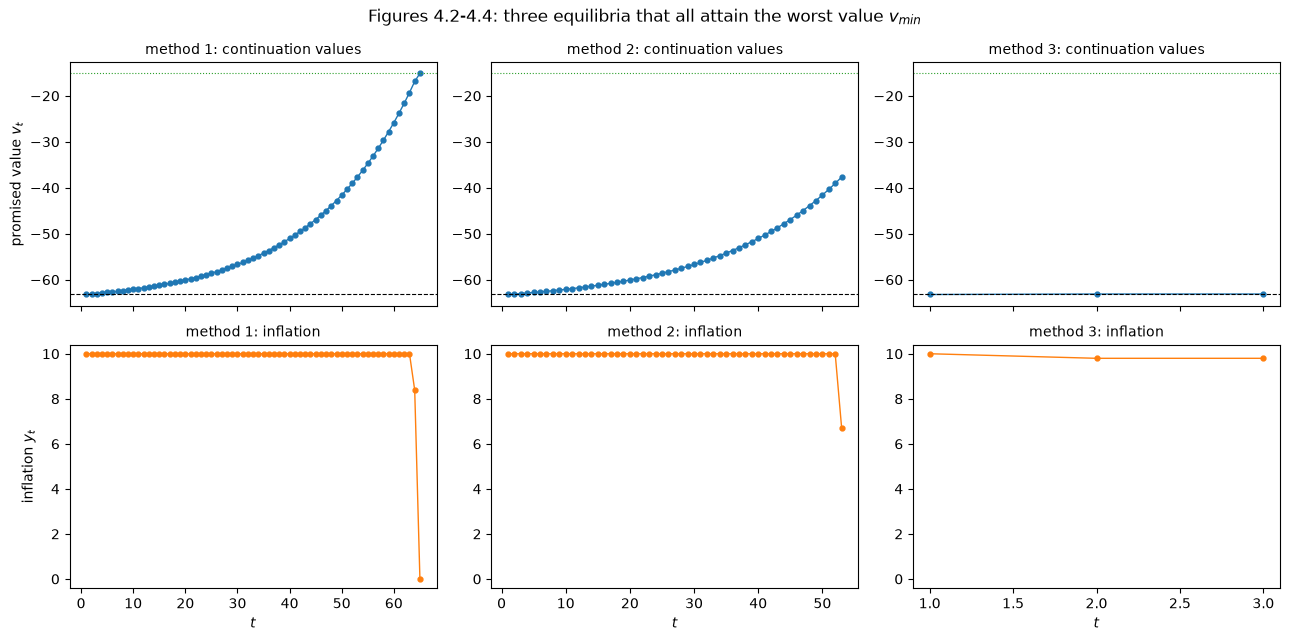
Fig. 93.2 Three subgame perfect equilibria that attain the same worst value#
print(f"Nash value {r_keep(m, y_nash(m)):.4f} at inflation {y_nash(m):.4f};  "
      f"worst value {v_lo:.4f}\n")
for name, (v, y) in paths.items():
    print(f"{name:9s}: {len(y):3d} periods before settling,  "
          f"first-period value {v[0]:.4f},  "
          f"terminal value {v[-1]:8.4f} at inflation {y[-1]:.4f}")
Nash value -38.7578 at inflation 6.8750;  worst value -63.2195

method 1 :  65 periods before settling,  first-period value -63.2195,  terminal value -15.1250 at inflation 0.0000
method 2 :  53 periods before settling,  first-period value -63.2195,  terminal value -37.6853 at inflation 6.7172
method 3 :   3 periods before settling,  first-period value -63.2195,  terminal value -63.1192 at inflation 9.7974
The three paths could hardly be less alike.
The first climbs at maximum inflation for about sixty periods before easing down to Ramsey.
The second climbs for a shorter spell and then freezes forever at a value just better than Nash, sustained by an inflation rate just below the Nash rate.
The third inflates at the maximum for a single period and then settles immediately, at a value barely above the worst one.
All three are subgame perfect, and all three deliver exactly the same value to the government.
The equilibrium concept has nothing to say about which of them describes the world.
93.8. Numerical example#
Here is the numerical example reported in chapter 4 of [Sargent, 1999], computed from scratch.
import pandas as pd

rows = [
    ("$\\theta$", m.θ, ""),
    ("$U^*$", m.U_star, ""),
    ("$y^\\#$", m.y_max, ""),
    ("$\\delta$", m.δ, ""),
    ("$y^N$ (Nash inflation)", y_nash(m), "6.8750"),
    ("$y^R$ (Ramsey inflation)", 0.0, "0"),
    ("$v^R$", r_keep(m, 0.0), "-15.1250"),
    ("$v^N$", r_keep(m, y_nash(m)), "-38.7578"),
    ("$\\underline v$", v_lo, "-63.2195"),
    ("$v_{\\rm abreu}$", abreu_value(m), "-17.6250"),
]
pd.DataFrame(rows, columns=["object", "computed", "reported in the book"]).set_index("object")
| computed | reported in the book | |
|---|---|---|
| object | ||
| $\theta$ | 1.250000 | |
| $U^*$ | 5.500000 | |
| $y^\#$ | 10.000000 | |
| $\delta$ | 0.950000 | |
| $y^N$ (Nash inflation) | 6.875000 | 6.8750 |
| $y^R$ (Ramsey inflation) | 0.000000 | 0 |
| $v^R$ | -15.125000 | -15.1250 |
| $v^N$ | -38.757812 | -38.7578 |
| $\underline v$ | -63.219512 | -63.2195 |
| $v_{\rm abreu}$ | -17.625000 | -17.6250 |
print(f"cutoff discount factor δ*        : {1 / (2 + m.θ**2):.4f}  (book reports 0.2807)")
print(f"Abreu stick-and-carrot at δ = 0.2: {abreu_value(m._replace(δ=0.2)):.4f}"
      f"  (book reports -55.125)")
cutoff discount factor δ*        : 0.2807  (book reports 0.2807)
Abreu stick-and-carrot at δ = 0.2: -55.1250  (book reports -55.125)
Every entry reproduces the book.
93.9. Interpretations#
The literature on credible plans bears mixed news for the triumph of natural-rate theory story of The Rise and Fall of U.S. Inflation.
It certainly rescues the government from the pessimism of The Credibility Problem: better outcomes than Nash are available, and at plausible discount factors Ramsey itself is an equilibrium.
But it rescues too much.
Values worse than Nash are equilibria too, and between the extremes lies a continuum.
The multitude of outcomes mutes the model empirically, and it undoes the very thing early rational-expectations researchers wanted from the hypothesis — the elimination of free parameters describing expectations.
93.9.1. Whose expectations are they?#
In his 1979 review of an OECD report edited by Paul McCracken, Lucas protested the report’s recommendation that “governments should try to promote good expectations,” as though expectations were an extra set of policy instruments.
In 1979 that protest was well aimed: rational-expectations models then took government policy as exogenous and made expectations a function of it, linked by cross-equation restrictions.
The theory of credible policy changes the picture in a way that vindicates neither side cleanly.
It turns systems of expectations into free parameters that influence outcomes — but into parameters that nobody inside the model gets to choose.
The government complies with equilibrium expectations about its own behavior.
Within an equilibrium, the government’s strategy is simultaneously a decision rule and a description of the public’s expectations, and the two cannot be disentangled.
As Sargent puts it: the authors of the McCracken report believed in multiplicity and manipulation, while Lucas doubted both; the literature on credible plans supports multiplicity but not manipulation.
93.9.2. Remedies#
Reputation alone is a weak foundation for anti-inflation policy, and that weakness has inspired proposals to change the game rather than to hope for a good equilibrium within it.
Rogoff [1985] proposed delegating monetary policy to someone who cares less about unemployment than society does.
Assigning it to someone unaware even of a temporary tradeoff would be equally effective, and Alan Blinder later suggested a related device: an authority who knows the natural rate and never wants unemployment to differ from it.
Maintaining a pool of potential central bankers with different inflation–unemployment preferences can also improve outcomes [Barro and Gordon, 1983].
93.9.3. Where this leaves us#
Every remedy just listed changes the institutions, not the theory.
Within the theory, the multiplicity is irreducible, and Sargent locates its source precisely: it stems from the rationality imputed to everyone in the system.
Perfection is what generates the continuum, because a system of expectations sophisticated enough to support one equilibrium is sophisticated enough to support many.
So the book retreats from perfection.
The remaining lectures replace fully rational participants with ones whose understanding of the economy is limited — first the public in Adaptive Expectations and the Phelps Problem, then both sides in Optimal Misspecified Beliefs and Self-Confirming Equilibria, and finally a government that estimates its model in real time in Adaptive Learning and Escape Dynamics.
Those models are closer to what Lucas had in mind when he criticized the McCracken report, and, unlike the theory of this lecture, they make predictions.
93.10. Exercises#
Exercise 93.1
The cutoff (93.11) claims that reversion to Nash sustains Ramsey forever if and only if \(\delta \geq 1/(2 + \theta^2)\) — a threshold that depends on the slope of the Phillips curve alone, and not on the natural rate \(U^*\) or the upper bound \(y^\#\).
Verify both claims numerically.
For a grid of \(\theta\) values, find the smallest \(\delta\) on a fine grid at which reversion to Nash supports Ramsey, and compare it with \(1/(2+\theta^2)\).
Then check that changing \(U^*\) leaves the answer untouched.
Solution
δ_grid = np.linspace(0.01, 0.99, 9801)

rows = []
for θ in (0.5, 1.0, 1.25, 2.0, 3.0):
    for U_star in (5.5, 11.0):
        md = Model(θ=θ, U_star=U_star)
        ok = [δ for δ in δ_grid
              if supports_ramsey_by_nash(md._replace(δ=δ))]
        rows.append((θ, U_star, min(ok), 1 / (2 + θ**2)))

pd.DataFrame(rows, columns=["$\\theta$", "$U^*$", "smallest $\\delta$ found",
                            "$1/(2+\\theta^2)$"]).round(4)
| $\theta$ | $U^*$ | smallest $\delta$ found | $1/(2+\theta^2)$ | |
|---|---|---|---|---|
| 0 | 0.50 | 5.5 | 0.4445 | 0.4444 |
| 1 | 0.50 | 11.0 | 0.4445 | 0.4444 |
| 2 | 1.00 | 5.5 | 0.3334 | 0.3333 |
| 3 | 1.00 | 11.0 | 0.3334 | 0.3333 |
| 4 | 1.25 | 5.5 | 0.2808 | 0.2807 |
| 5 | 1.25 | 11.0 | 0.2808 | 0.2807 |
| 6 | 2.00 | 5.5 | 0.1667 | 0.1667 |
| 7 | 2.00 | 11.0 | 0.1667 | 0.1667 |
| 8 | 3.00 | 5.5 | 0.0910 | 0.0909 |
| 9 | 3.00 | 11.0 | 0.0910 | 0.0909 |
The grid search matches the closed form to within the grid spacing, and doubling \(U^*\) changes nothing.
The reason both \(U^*\) and \(y^\#\) drop out is visible in (93.4): the one-period temptation at \(y = 0\) and the Nash–Ramsey value gap are both proportional to \(U^{*2}\), so the scale cancels from the inequality, and \(y^\#\) never enters because neither side involves the upper bound.
A steeper Phillips curve — a larger \(\theta\) — makes the Nash outcome worse relative to Ramsey, which strengthens the threat and lets a less patient government be held at zero inflation.
Exercise 93.2
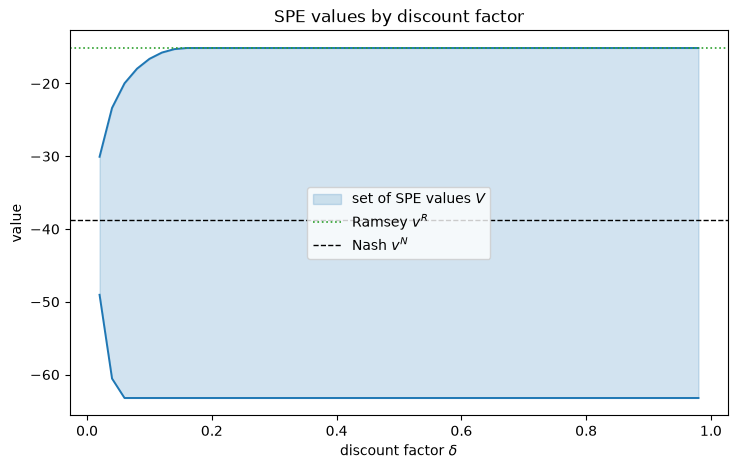
The set of equilibrium values shrinks as the government becomes impatient.
Use solve_aps to compute the set \(V = [\underline v, \overline v]\) for a grid of discount
factors, and plot both endpoints against \(\delta\), marking the Nash and Ramsey values.
At roughly what discount factor does the best equilibrium value stop being Ramsey?
What happens to the set as \(\delta \to 0\), and why is that the answer you should expect?
Solution
δs = np.linspace(0.02, 0.98, 49)
lows, highs = [], []
for δ in δs:
    Wδ, _ = solve_aps(m._replace(δ=δ))
    lows.append(Wδ[0])
    highs.append(Wδ[1])

fig, ax = plt.subplots(figsize=(8.5, 5))
ax.fill_between(δs, lows, highs, alpha=0.2, color='C0', label='set of SPE values $V$')
ax.plot(δs, highs, 'C0', lw=1.4)
ax.plot(δs, lows, 'C0', lw=1.4)
ax.axhline(r_keep(m, 0.0), color='C2', ls=':', lw=1.2, label='Ramsey $v^R$')
ax.axhline(r_keep(m, y_nash(m)), color='k', ls='--', lw=1, label='Nash $v^N$')
ax.set_xlabel(r'discount factor $\delta$')
ax.set_ylabel('value')
ax.set_title('SPE values by discount factor')
ax.legend()
plt.show()
best_is_ramsey = [δ for δ, h in zip(δs, highs)
                  if np.isclose(h, r_keep(m, 0.0), atol=1e-6)]
print(f"best value equals Ramsey for δ ≥ {min(best_is_ramsey):.3f}")
print(f"closed-form cutoff for Nash reversion: δ* = {1/(2+m.θ**2):.3f}")
best value equals Ramsey for δ ≥ 0.180
closed-form cutoff for Nash reversion: δ* = 0.281
The best equilibrium value equals Ramsey down to a discount factor well below the \(\delta^\star \approx 0.28\) of (93.11), and the reason is Abreu.
The cutoff \(\delta^\star\) was derived using reversion to Nash as the threat; the APS set uses the worst equilibrium as the threat, which is a good deal harsher, so Ramsey survives at lower discount factors than Barro and Gordon’s argument alone would suggest.
As \(\delta \to 0\) the set collapses toward the single point \(v^N\).
That is what it must do: an entirely impatient government cares only about the current period, promises about the future carry no weight, and the only outcome that can be sustained is the one the government would choose myopically — the Nash outcome.
Exercise 93.3
Method 3 in the multiplicity section is the boldest of the three: it inflates at \(y^\#\) for a single period and then freezes forever at a constant inflation rate.
Because it settles immediately, its incentive constraint is the tightest of the three, so it is worth checking rather than assuming.
Verify directly that method 3 is a subgame perfect equilibrium: confirm that its first-period promise is honoured, that its frozen continuation value lies inside \(V\), and that the government prefers adherence to deviation in both phases, using \(\underline v\) as the punishment.
Solution
v_2 = next_value(m, v_lo)
y_tilde = action_delivering(m, v_2)

# phase 1: promised v_lo, prescribed action y^#, continuation v_2 on adherence
lhs_1 = (1 - m.δ) * r_keep(m, m.y_max) + m.δ * v_2
rhs_1 = (1 - m.δ) * r_cheat(m, m.y_max) + m.δ * v_lo

# phase 2: promised v_2, prescribed action ỹ, continuation v_2 on adherence
lhs_2 = (1 - m.δ) * r_keep(m, y_tilde) + m.δ * v_2
rhs_2 = (1 - m.δ) * r_cheat(m, y_tilde) + m.δ * v_lo

print(f"v_2 = {v_2:.4f},  ỹ = {y_tilde:.4f}")
print(f"v_2 lies inside V = [{v_lo:.4f}, {v_hi:.4f}]: "
      f"{v_lo <= v_2 <= v_hi}")
print(f"phase 1 delivers the promise: {np.isclose(lhs_1, v_lo)}")
print(f"phase 1 incentive: {lhs_1:.4f} >= {rhs_1:.4f}  ->  {lhs_1 >= rhs_1}")
print(f"phase 2 delivers the promise: {np.isclose(lhs_2, v_2)}")
print(f"phase 2 incentive: {lhs_2:.4f} >= {rhs_2:.4f}  ->  {lhs_2 >= rhs_2}")
print(f"slack in phase 2: {lhs_2 - rhs_2:.6f}")
v_2 = -63.1192,  ỹ = 9.7974
v_2 lies inside V = [-63.2195, -15.1250]: True
phase 1 delivers the promise: True
phase 1 incentive: -63.2195 >= -63.2195  ->  True
phase 2 delivers the promise: True
phase 2 incentive: -63.1192 >= -63.1312  ->  True
slack in phase 2: 0.011955
All the conditions hold, and the first-period promise is delivered exactly.
The margin in the second phase is very thin, and that is not an accident.
The frozen value \(v_2\) is only barely above \(\underline v\), so the punishment for deviating is only barely worse than the equilibrium itself — which is precisely what it means to be near the bottom of the set of equilibrium values.
Push the construction any lower and the incentive constraint fails, which is another way of seeing why \(\underline v\) is where it is.