87. Exchange Rate Indeterminacy, Learning, and Experiments#
87.1. Overview#
In A Peculiar Definition of Bounded Rationality we met a model in which rational expectations cannot pin down the exchange rate at all.
Two fiat currencies, perfect substitutes as long as their rates of return are equal, leave the exchange rate \(e\) completely unrestricted: if the equilibrium conditions have a solution for one \(e\), they have a solution for every other, and the real allocation is identical across all of them.
This lecture, following Sargent [1993], expels the rational agents from that economy and puts adaptive ones in their place.
Two questions organize what follows.
First, does learning pin the exchange rate down?
An adaptive agent has beliefs, a rule for revising them, and initial conditions, and those initial conditions are exactly what the equilibrium conditions failed to determine.
So a system of adaptive agents can select an exchange rate where rational expectations could not.
We shall see that it does, but in a very particular way.
Newton–Raphson learners converge to a determinate exchange rate that depends entirely on where they started.
The “dead hand of history” does the pinning that fundamentals refused to do.
Second, does a ghost of the indeterminacy survive?
It does.
The rest points of the learning algorithm reproduce the indeterminacy exactly: the condition that stops the algorithm is the same arbitrage condition that made the exchange rate free in the first place.
Sargent calls a regime that leaves the exchange rate history-dependent “a weak reed” on which to base exchange rate determination.
Then we turn to evidence.
Arifovic [1996] ran this economy as a laboratory experiment with paying human subjects.
Their exchange rate never settled down.
And when she replaced the Newton–Raphson learners with a genetic algorithm — a population of binary-string agents bred by selection, crossover, and mutation — she got an economy whose exchange rate wanders persistently, with a spectrum resembling real floating exchange rates.
That contrast — a learning rule that converges versus one that generates permanent volatility — is where this lecture lands, and it is the on-ramp to Money as a Medium of Exchange among Artificially Intelligent Agents, where genetic algorithms and classifier systems take over entirely.
Let’s start with some imports.
import numpy as np
import pandas as pd
import matplotlib.pyplot as plt
from typing import NamedTuple
87.2. The two-currency economy#
We use the overlapping generations incarnation of the Kareken and Wallace [1981] indeterminacy.
At each date \(t\), \(N\) two-period-lived agents are born, endowed with \(w_1\) when young and \(w_2\) when old, with \(w_1 > w_2\).
There are two fiat currencies in fixed supplies \(H_1\) and \(H_2\).
A young agent makes two decisions: how much to save, \(s_t\), and what fraction \(\lambda_t\) of that saving to hold in currency 1 (the rest going to currency 2).
The realized lifetime utility of an agent who chooses \((s_t, \lambda_t)\) is
where \(p_{it}\) is the price level in currency \(i\) and \(p_{it}/p_{i,t+1}\) is the gross return on holding currency \(i\).
We take \(u(c) = \ln c\) throughout.
Equating each currency’s supply to the demand for it gives the price levels
and the exchange rate is \(e_t = p_{1t}/p_{2t}\).
87.2.1. The indeterminacy, recalled#
Consider a stationary equilibrium with constant prices.
Then each currency returns \(p_{it}/p_{i,t+1} = 1\), so both returns are equal, and the portfolio return in (87.1) is \(1\) regardless of \(\lambda\).
The saving decision then solves \(\max_s \ln(w_1 - s) + \ln(w_2 + s)\), giving
but the portfolio share \(\lambda\) is completely undetermined: utility does not depend on it when the two returns are equal.
And \(\lambda\) is what fixes the exchange rate.
From (87.2), with a common \((s, \lambda)\),
Every \(\lambda \in (0, 1)\) is an equilibrium, so every \(e \in (0, \infty)\) is an equilibrium.
This is the indeterminacy of A Peculiar Definition of Bounded Rationality, now expressed through an undetermined portfolio choice.
This lecture runs two economies with different parameters — Sargent’s and Arifovic’s — so we carry the parameters in a container and pass them explicitly rather than leaving them lying about as globals.
class Params(NamedTuple):
    w1: float          # endowment when young
    w2: float          # endowment when old
    H1: float          # fixed supply of currency 1
    H2: float          # fixed supply of currency 2

    @property
    def s_star(self):
        "Rational expectations saving rate, when both currencies return 1."
        return (self.w1 - self.w2) / 2


kw = Params(w1=20.0, w2=15.0, H1=100.0, H2=120.0)

print(f"rational expectations saving rate s* = {kw.s_star}")
print(f"any portfolio share λ is an equilibrium, and e = (H1/H2)(1-λ)/λ is free")
rational expectations saving rate s* = 2.5
any portfolio share λ is an equilibrium, and e = (H1/H2)(1-λ)/λ is free
87.3. Newton–Raphson learning#
Now expel the rational agents.
Following Sargent [1993], we split the population into two classes — call them “even” and “odd” — because a cohort’s lifetime utility cannot be evaluated until it is old.
Each class carries its own rule \((s, \lambda)\), updated only from the experience of earlier agents of the same class.
An agent revises \((s, \lambda)\) by a Newton–Raphson step against realized utility: move in the direction that a second-order expansion of (87.1) says would have raised utility, given the returns the agent actually experienced.
Writing \(g\) for the gradient and \(R\) for a running estimate of the (negative-definite) Hessian, the recursion is
with \(H_\tau\) the realized Hessian and \(\gamma_\tau\) a gain.
Here is the gradient and Hessian of (87.1) in the returns \(R_1 = p_{1t}/p_{1,t+1}\) and \(R_2 = p_{2t}/p_{2,t+1}\).
def grad_hess(p, s, lam, R1, R2):
    "Gradient and Hessian of realized utility U(s, λ)."
    A = lam*R1 + (1 - lam)*R2               # portfolio gross return
    c2 = p.w2 + s*A                         # old-age consumption
    dR = R1 - R2
    g = np.array([-1/(p.w1 - s) + A/c2,
                  s*dR/c2])
    H_ss = -1/(p.w1 - s)**2 - A**2/c2**2
    H_ll = -s**2 * dR**2 / c2**2
    H_sl = dR/c2 - s*A*dR/c2**2
    return g, np.array([[H_ss, H_sl], [H_sl, H_ll]])
87.3.1. The indeterminacy shows up as a singular Hessian#
Look at the \(\lambda\) block of the Hessian.
When the two returns are equal, \(R_1 = R_2\), every \(\lambda\)-derivative vanishes: the gradient component \(s(R_1 - R_2)/c_2\) is zero, and so is the curvature \(-s^2(R_1 - R_2)^2/c_2^2\).
Utility is flat in \(\lambda\) at equal returns.
That is the indeterminacy, seen locally: there is no force pushing \(\lambda\) in any direction, so a Newton step — which divides the gradient by the curvature — is \(0/0\) in the \(\lambda\) direction.
For the algorithm to move at all we must keep \(R\) invertible.
We do that with a small prior curvature \(\kappa\) in the \(\lambda\) direction.
Economically this is exactly the sluggishness that Sargent [1993] invokes: it is the “dead hand of history” that lets an otherwise-free exchange rate settle down.
def newton_learning(p, s0, lam0, T=400, gain=0.3, κ=0.5):
    """
    Two-currency OLG with Newton-Raphson learning of (s, λ), one rule per class
    (even/odd).  κ is a prior curvature in the indeterminate λ direction that
    keeps the second-moment matrix R invertible.
    """
    s = np.array(s0, float)
    lam = np.array(lam0, float)
    R = [np.array([[-1.0, 0.0], [0.0, -κ]]) for _ in range(2)]   # prior curvature
    p1 = np.empty(T)
    p2 = np.empty(T)
    e = np.empty(T)
    s_hist = np.empty((T, 2))
    lam_hist = np.empty((T, 2))

    for t in range(T):
        j = t % 2                                    # class that is young at t
        p1[t] = p.H1 / (lam[j]*s[j])
        p2[t] = p.H2 / ((1 - lam[j])*s[j])
        e[t] = p1[t] / p2[t]
        if t >= 1:                                   # class young at t-1 is now old
            jp = 1 - j
            R1, R2 = p1[t-1]/p1[t], p2[t-1]/p2[t]
            g, H = grad_hess(p, s[jp], lam[jp], R1, R2)
            H[1, 1] -= κ                         # retain prior λ-curvature
            R[jp] = R[jp] + gain*(H - R[jp])
            step = gain * np.linalg.solve(R[jp], g)
            s[jp] = np.clip(s[jp] - step[0], 0.1, p.w1 - 0.1)
            lam[jp] = np.clip(lam[jp] - step[1], 0.02, 0.98)
        s_hist[t] = s
        lam_hist[t] = lam

    return e, s_hist, lam_hist
87.3.2. Convergence to a history-dependent exchange rate#
Run two experiments that are identical except for the initial portfolio shares.
e1, s1, l1 = newton_learning(kw, [3.5, 2.0], [0.35, 0.40])
e2, s2, l2 = newton_learning(kw, [2.0, 3.5], [0.62, 0.58])

fig, axes = plt.subplots(1, 3, figsize=(14, 4))

axes[0].plot(np.log(e1), 'C0', lw=1.3, label="experiment 1")
axes[0].plot(np.log(e2), 'C1', lw=1.3, label="experiment 2")
axes[0].set_title("log exchange rate")
axes[0].set_xlabel("$t$")
axes[0].legend(frameon=False)

for s_h, c in [(s1, 'C0'), (s2, 'C1')]:
    axes[1].plot(s_h[:, 0], color=c, lw=1.0)
    axes[1].plot(s_h[:, 1], color=c, lw=1.0, ls=':')
axes[1].axhline(kw.s_star, color='k', lw=0.8, ls='--')
axes[1].set_title("saving  (solid = even, dotted = odd)")
axes[1].set_xlabel("$t$")

for l_h, c in [(l1, 'C0'), (l2, 'C1')]:
    axes[2].plot(l_h[:, 0], color=c, lw=1.0)
    axes[2].plot(l_h[:, 1], color=c, lw=1.0, ls=':')
axes[2].set_title(r"portfolio share $\lambda$")
axes[2].set_xlabel("$t$")
plt.tight_layout()
plt.show()
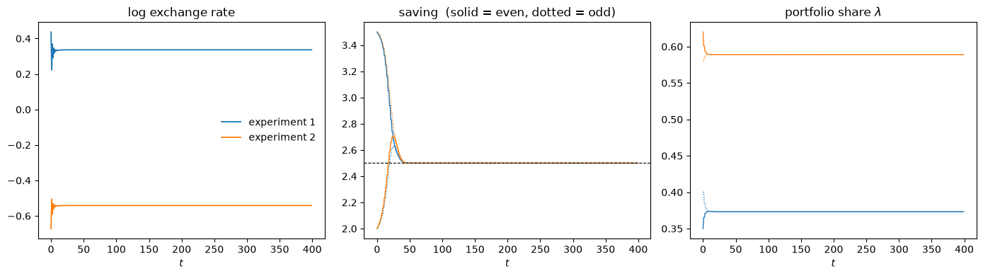
Fig. 87.1 Newton-Raphson learning from two initial conditions#
Both economies converge.
Saving climbs or falls to the rational expectations rate \(s^\star = 2.5\) from either side, and the two classes’ portfolio shares merge to a common value.
But the two experiments converge to different exchange rates.
The only thing that differed between them was where the portfolios started.
for name, e, l in [("experiment 1", e1, l1), ("experiment 2", e2, l2)]:
    print(f"{name}: e → {e[-1]:.4f},  s → {s1[-1][0]:.3f},  λ → {l[-1][0]:.3f}")
experiment 1: e → 1.3998,  s → 2.500,  λ → 0.373
experiment 2: e → 0.5819,  s → 2.500,  λ → 0.589
The saving rate is pinned down by fundamentals; the exchange rate is pinned down by history.
87.3.3. The dead hand of history#
To see how completely history governs the outcome, sweep the initial portfolio share and record the exchange rate each economy settles on.
λ0_grid = np.linspace(0.15, 0.85, 15)
e_limits = [newton_learning(kw, [4.0, 4.0], [λ0, λ0])[0][-1] for λ0 in λ0_grid]

fig, ax = plt.subplots(figsize=(7, 4.5))
ax.plot(λ0_grid, e_limits, 'C0o-', ms=5, label="limiting $e$ from learning")
ax.plot(λ0_grid, (kw.H1/kw.H2)*(1 - λ0_grid)/λ0_grid, 'k--', lw=1,
        label=r"$(H_1/H_2)(1-\lambda)/\lambda$")
ax.set_xlabel(r"initial portfolio share $\lambda_0$")
ax.set_ylabel("limiting exchange rate $e$")
ax.legend(frameon=False)
plt.show()
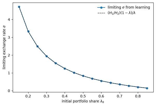
Fig. 87.2 Limiting exchange rate against initial portfolio share#
The limiting exchange rate traces out the entire rational expectations continuum.
Every point on the curve is a valid rational expectations equilibrium; learning selects among them purely by initial condition.
This is the sense in which learning renders the exchange rate determinate.
It does not add a fundamental that fundamentals were missing.
It converts an indeterminacy of levels into a dependence on history: the exchange rate the economy reaches is whatever the initial portfolio beliefs implied, frozen in place.
87.3.4. The ghost of indeterminacy#
Why does the exchange rate freeze rather than move to some particular value?
Because the algorithm comes to rest wherever the gradient vanishes, and the portfolio gradient \(s(R_1 - R_2)/c_2\) vanishes precisely when \(R_1 = R_2\), the arbitrage condition that made the exchange rate free under rational expectations.
# at the limit the classes have merged, so prices are constant and R1 = R2 = 1
s_lim, lam_lim = s1[-1], l1[-1]
p1_lim = kw.H1 / (lam_lim*s_lim)
p2_lim = kw.H2 / ((1 - lam_lim)*s_lim)
print(f"classes converged to a common rule:  s = {s_lim.round(4)},  λ = {lam_lim.round(4)}")
print(f"→ prices constant across periods, so R1 = R2 = 1 (arbitrage holds at the rest point)")
print(f"→ the λ-gradient is zero for *any* λ, so learning cannot move the exchange rate off "
      f"wherever history left it")
classes converged to a common rule:  s = [2.5 2.5],  λ = [0.3732 0.3732]
→ prices constant across periods, so R1 = R2 = 1 (arbitrage holds at the rest point)
→ the λ-gradient is zero for *any* λ, so learning cannot move the exchange rate off wherever history left it
The rest points of the learning dynamics are the rational expectations equilibria, exchange rate and all.
The indeterminacy is not resolved; it is displaced into the initial conditions.
Sargent is blunt about how much weight this can bear:
Put differently, a regime that allows the exchange rate to be history-dependent seems to be an ill-formed mechanism.
An exchange rate determined by nothing but the accident of initial beliefs is a weak reed.
If the economy is a shade different — if the learning rule keeps experimenting rather than settling — the whole construction can come apart.
That is exactly what the next two exhibits show.
87.4. Evidence from the laboratory#
Arifovic [1996] implemented this two-currency economy as an experiment with paying human subjects, using \(w_1 = 11\), \(w_2 = 1\), \(H_1 = H_2 = 10\).
Each young subject chose a saving rate and a fraction to allocate between the two currencies; the experimenters cleared the two money markets against those choices, exactly as in (87.2).
The result did not look like the Newton–Raphson simulations at all.
The exchange rate fluctuated persistently, roughly within a band from \(0.5\) to \(2\), and showed no sign of settling down.
If anything the amplitude grew across sessions.
The simple Newton–Raphson model, which always converges to a constant, does a poor job of matching that.
So Arifovic built a different model of the same economy, one in which the agents are a population bred by a genetic algorithm.
87.5. A genetic algorithm economy#
Now each class is a population of \(N = 30\) agents, and each agent is a binary string of length \(30\): the first \(20\) bits encode its saving rate, the last \(10\) its portfolio share.
Every period the young population’s strings are decoded into \((s_i, \lambda_i)\) pairs, the two money markets clear against the aggregates via (87.2), and the exchange rate is read off.
A generation later, when the cohort is old, each string’s realized utility (87.1) is its fitness, and the genetic algorithm breeds the next generation.
N, L_s, L_lam = 30, 20, 10           # population size; bits for saving and portfolio

arifovic = Params(w1=11.0, w2=1.0, H1=10.0, H2=10.0)

def decode(p, pop):
    "Binary strings → (s, λ), with s in (0, w1) and λ in (0, 1)."
    ints_s = pop[:, :L_s] @ (1 << np.arange(L_s)[::-1])
    ints_l = pop[:, L_s:] @ (1 << np.arange(L_lam)[::-1])
    s = 0.05 + (p.w1 - 0.10) * ints_s / (2**L_s - 1)
    lam = 0.02 + 0.96 * ints_l / (2**L_lam - 1)
    return s, lam

def market_prices(p, pop):
    s, lam = decode(p, pop)
    return p.H1 / np.sum(lam*s), p.H2 / np.sum((1 - lam)*s)

def fitness(p, pop, R1, R2):
    "Realized lifetime utility of each string given the returns it experienced."
    s, lam = decode(p, pop)
    c2 = p.w2 + s*(lam*R1 + (1 - lam)*R2)
    return np.log(p.w1 - s) + np.log(np.maximum(c2, 1e-9))
The genetic algorithm has the classic three operators — fitness-proportional selection of parents, single-point crossover, and bit-flip mutation — plus one that Arifovic introduced, the election operator: a child is admitted to the next generation only if it would have been fitter than its parent on the most recent returns, otherwise the parent survives.
def genetic_step(p, pop, R1, R2, rng, p_mut=0.033, election=True):
    "Breed one new generation from the current one."
    fit = fitness(p, pop, R1, R2)
    weight = fit - fit.min() + 1e-6                  # shift to positive for roulette wheel
    new = np.empty_like(pop)
    for k in range(0, N, 2):
        i, j = np.searchsorted(np.cumsum(weight), rng.random(2) * weight.sum())
        parents = np.array([pop[i], pop[j]])
        cut = rng.integers(1, L_s + L_lam)           # single-point crossover
        kids = parents.copy()
        kids[0, cut:], kids[1, cut:] = parents[1, cut:], parents[0, cut:]
        for c in kids:                               # mutation
            c[rng.random(L_s + L_lam) < p_mut] ^= 1
        if election:                                 # Arifovic's election operator
            f_kids = fitness(p, kids, R1, R2)
            f_par = fitness(p, parents, R1, R2)
            for m in range(2):
                new[k + m] = kids[m] if f_kids[m] > f_par[m] else parents[m]
        else:
            new[k], new[k + 1] = kids
    return new


def genetic_economy(p, T=3000, seed=0, election=True):
    rng = np.random.default_rng(seed)
    pops = [rng.integers(0, 2, (N, L_s + L_lam)) for _ in range(2)]   # even, odd
    p1 = np.empty(T)
    p2 = np.empty(T)
    e = np.empty(T)
    for t in range(T):
        j = t % 2
        p1[t], p2[t] = market_prices(p, pops[j])
        e[t] = p1[t] / p2[t]
        if t >= 1:
            jp = 1 - j
            R1, R2 = p1[t-1]/p1[t], p2[t-1]/p2[t]
            pops[jp] = genetic_step(p, pops[jp], R1, R2, rng, election=election)
    return e
87.5.1. Volatility that never dies#
e_ga = genetic_economy(arifovic, T=4000, seed=1)
log_e = np.log(e_ga[500:])                            # drop a burn-in

fig, ax = plt.subplots(figsize=(9, 4))
ax.plot(log_e, lw=0.5)
ax.set_xlabel("$t$")
ax.set_ylabel("$\\log e_t$")
plt.show()
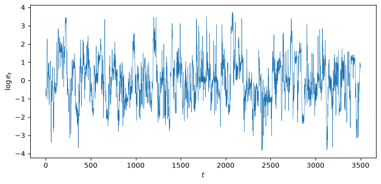
Fig. 87.3 Exchange rate in the genetic-algorithm economy#
The exchange rate wanders and keeps wandering.
Unlike the Newton–Raphson learner, the genetic population never settles: mutation keeps injecting new strings, and the market keeps repricing them.
The volatility is a permanent feature, not a transient.
early = np.log(e_ga[500:1500]).std()
late = np.log(e_ga[3000:]).std()
print(f"standard deviation of log e, early window: {early:.3f}")
print(f"standard deviation of log e, late window:  {late:.3f}")
print("→ the volatility does not damp out over time")
standard deviation of log e, early window: 1.279
standard deviation of log e, late window:  1.194
→ the volatility does not damp out over time
87.5.2. The shape of the volatility#
Arifovic reported that the exchange rate in her genetic economy behaves almost like a random walk — but with mean reversion, showing up as a dip in the spectrum of its first difference at zero frequency.
def averaged_spectrum(x, n_seg=16):
    "Bartlett-averaged periodogram, for a readable spectral estimate."
    x = x - x.mean()
    seg = len(x) // n_seg
    acc = np.zeros(seg // 2 + 1)
    for k in range(n_seg):
        acc += np.abs(np.fft.rfft(x[k*seg:(k+1)*seg]))**2 / seg
    return np.fft.rfftfreq(seg), acc / n_seg


d_log_e = np.diff(np.log(e_ga[500:]))
d_log_e = np.clip(d_log_e, *np.percentile(d_log_e, [1, 99]))    # winsorize tails
freq, spec = averaged_spectrum(d_log_e)

def acf(x, K):
    x = x - x.mean()
    return np.array([np.sum(x[k:]*x[:len(x)-k]) / np.sum(x*x) for k in range(K)])


fig, axes = plt.subplots(1, 2, figsize=(12, 4))
axes[0].plot(freq[1:], spec[1:], lw=1.2)
axes[0].axhline(spec[1:].mean(), color='k', ls=':', lw=0.8)
axes[0].set_title(r"spectrum of $\Delta \log e$")
axes[0].set_xlabel("frequency")

axes[1].bar(range(25), acf(np.log(e_ga[500:]), 25))
axes[1].set_title(r"autocorrelation of $\log e$")
axes[1].set_xlabel("lag")
plt.tight_layout()
plt.show()
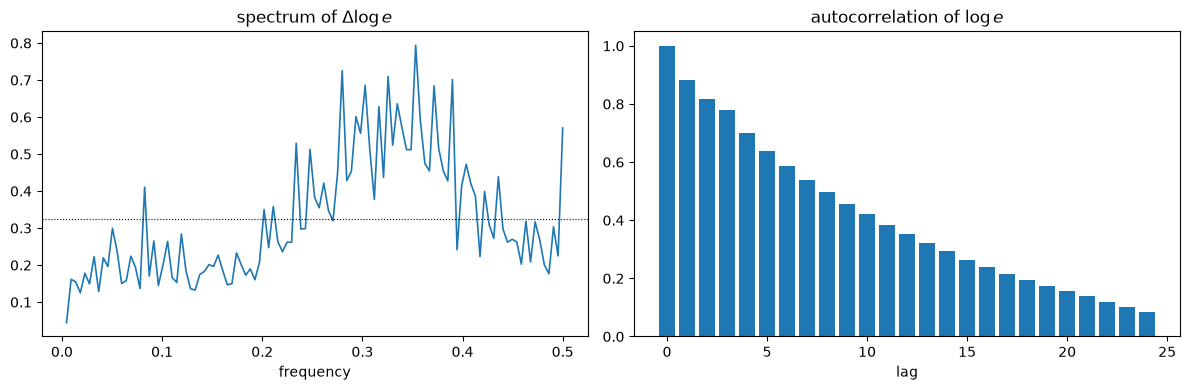
Fig. 87.4 Spectrum and autocorrelation of the exchange rate#
The spectrum of the first difference is low near zero frequency and rises toward the higher frequencies, the signature of a series whose level is close to a random walk, but with enough mean reversion to pull the low-frequency power down.
The autocorrelation of the level decays slowly, as a near-unit-root series would, but it does decay, which a pure random walk’s would not.
band = slice(1, len(spec)//2)
print(f"spectral power of Δlog e near zero frequency: {spec[1]:.4f}")
print(f"average spectral power over low-to-mid band:  {spec[band].mean():.4f}")
print(f"→ pronounced dip at zero frequency (mean reversion): {spec[1] < spec[band].mean()}")
spectral power of Δlog e near zero frequency: 0.0446
average spectral power over low-to-mid band:  0.2174
→ pronounced dip at zero frequency (mean reversion): True
The book’s assessment: real floating exchange rates for hard-currency pairs have spectra of log differences that look much like this, except without the dip at zero frequency; actual exchange rates are even closer to pure random walks.
Arifovic’s genetic economy, with no fundamental shocks at all, manufactures most of the way there out of nothing but a population of adapting agents repricing two intrinsically identical currencies.
87.6. Concluding remarks#
Two models of the same indeterminate economy gave two very different verdicts.
The Newton–Raphson learner converges — and in converging, exposes the indeterminacy rather than curing it.
Its rest point is an arbitrage condition that leaves the exchange rate free, so the limiting exchange rate is whatever history’s initial portfolio beliefs implied.
Determinacy by dead hand, which Sargent judges a weak reed.
The genetic-algorithm economy does not converge.
A whole population of adapting strings, constantly refreshed by mutation and repriced by the market, generates exchange rate volatility that never dies and that mimics the low-frequency behavior of real floating rates — from an economy with no fundamental disturbances whatsoever.
The gap between them is not about the economics, which is identical, but about the adaptive machinery.
A device that stabilizes a single agent’s learning — the election operator, which keeps only improving offspring — turns out, inside a self-referential market, to sustain volatility rather than damp it (Exercise 87.2).
Which learning model an economist reaches for is, once again, one of the choices that the bounded-rationality program forces into the open.
That machinery — Holland’s genetic algorithm, and its richer cousin the classifier system — is the subject of Money as a Medium of Exchange among Artificially Intelligent Agents, where a population of adaptive agents must not merely tune a portfolio but discover from scratch which good will serve as money.
87.7. Exercises#
Exercise 87.1
The Newton–Raphson economy converges to a rest point where the two classes share a common rule and the arbitrage condition \(R_1 = R_2\) holds.
Verify the claim that the limiting exchange rate depends on the whole initial condition, not just the initial \(\lambda\), by starting the two classes asymmetrically.
Run the learner from several initial conditions in which the even and odd classes begin with different portfolio shares, and confirm that (a) the classes’ shares merge to a common value, (b) saving converges to \(s^\star\), and © the limiting exchange rate depends on the starting point.
Does the common limiting \(\lambda\) equal the average of the two initial shares?
Solution
rows = []
starts = [([3.0, 2.2], [0.30, 0.50]),
          ([2.2, 3.0], [0.50, 0.30]),
          ([3.5, 2.0], [0.35, 0.55]),
          ([2.5, 2.5], [0.40, 0.60])]
for s0, lam0 in starts:
    e, s_h, l_h = newton_learning(kw, s0, lam0, T=600)
    rows.append([str(lam0), l_h[-1][0], l_h[-1][1], s_h[-1].mean(),
                 e[-1], np.mean(lam0)])

pd.DataFrame(rows, columns=["initial λ", "λ even (limit)", "λ odd (limit)",
                            "s (limit)", "e (limit)", "mean of initial λ"]).round(4)
| initial λ | λ even (limit) | λ odd (limit) | s (limit) | e (limit) | mean of initial λ | |
|---|---|---|---|---|---|---|
| 0 | [0.3, 0.5] | 0.4117 | 0.4117 | 2.5 | 1.1908 | 0.40 |
| 1 | [0.5, 0.3] | 0.3666 | 0.3666 | 2.5 | 1.4397 | 0.40 |
| 2 | [0.35, 0.55] | 0.4433 | 0.4433 | 2.5 | 1.0463 | 0.45 |
| 3 | [0.4, 0.6] | 0.5208 | 0.5208 | 2.5 | 0.7668 | 0.50 |
The two classes’ shares always merge (columns 2 and 3 agree), saving always converges to \(s^\star = 2.5\), and the limiting exchange rate differs across starting points — so it is genuinely history-dependent.
But the common limiting \(\lambda\) is not simply the average of the two initial shares: compare the merged value with the last column.
The transient path matters, because while the classes still differ the returns differ, and those transient return gaps push \(\lambda\) around before the arbitrage condition shuts the motion off.
The exchange rate records the whole history of the adjustment, not just its starting average.
Exercise 87.2
Arifovic’s election operator admits a child to the next generation only if it beats its parent on the latest returns.
In single-agent optimization such a filter can only help — it never lets a worse rule replace a better one.
But this economy is self-referential: the returns against which fitness is measured are themselves determined by the population’s choices.
Investigate what the election operator does to exchange rate volatility.
Run the genetic economy with and without it across several seeds, and report the volatility of the log exchange rate.
Which way does the operator push volatility, and can you explain why?
Solution
rows = []
for election in (True, False):
    sds = [np.log(genetic_economy(arifovic, T=2500, seed=sd,
                                  election=election)[500:]).std()
           for sd in range(6)]
    rows.append([election, np.mean(sds), np.min(sds), np.max(sds)])

pd.DataFrame(rows, columns=["election operator", "mean s.d. of log e",
                            "min", "max"]).round(3)
| election operator | mean s.d. of log e | min | max | |
|---|---|---|---|---|
| 0 | True | 1.220 | 1.081 | 1.350 |
| 1 | False | 0.522 | 0.473 | 0.553 |
The election operator raises volatility — the opposite of its stabilizing role in single-agent search.
The mechanism is the self-reference.
With the filter on, the population keeps only offspring that beat their parents on last period’s returns, so it chases the recently profitable portfolio.
But “recently profitable” depends on the exchange rate, which the population’s own chasing moves — so the whole population piles into the recent winner, overshoots, and the exchange rate lurches to make a different portfolio profitable, whereupon the population chases that.
Without the filter, mutation keeps the population diffuse, and diverse portfolios partly cancel in the aggregates (87.2), damping the swings.
A device that unambiguously improves an isolated learner can destabilize a market of learners.
It is a compact warning about reading single-agent intuitions into multi-agent systems — a theme that returns in Money as a Medium of Exchange among Artificially Intelligent Agents.
Exercise 87.3
The lecture claimed the genetic economy’s exchange rate is “close to a random walk, but with mean reversion.”
Make the claim quantitative.
Treating \(\log e_t\) as data, estimate the first-order autoregressive coefficient in \(\log e_t = \mu + \phi \log e_{t-1} + \varepsilon_t\), and compare it with \(1\) (a pure random walk).
Do this for several seeds.
Is \(\phi\) close to but below \(1\), consistent with a near-unit-root, mean-reverting series?
Solution
def ar1_coefficient(x):
    "OLS estimate of φ in x_t = μ + φ x_{t-1} + ε."
    x0, x1 = x[:-1], x[1:]
    X = np.column_stack([np.ones_like(x0), x0])
    μ, φ = np.linalg.lstsq(X, x1, rcond=None)[0]
    return φ

rows = []
for sd in range(6):
    le = np.log(genetic_economy(arifovic, T=3000, seed=sd)[500:])
    rows.append([sd, ar1_coefficient(le)])

table = pd.DataFrame(rows, columns=["seed", "AR(1) coefficient φ"])
print(table.round(4).to_string(index=False))
print(f"\nmean φ across seeds: {table['AR(1) coefficient φ'].mean():.4f}")
 seed  AR(1) coefficient φ
    0               0.9165
    1               0.8849
    2               0.8974
    3               0.8739
    4               0.8726
    5               0.8979

mean φ across seeds: 0.8905
The estimated \(\phi\) is consistently close to \(1\) but strictly below it — a highly persistent series that nonetheless reverts to its mean rather than drifting forever.
That is precisely the “near random walk with mean reversion” the spectrum showed: a pure random walk would have \(\phi = 1\) exactly (and no dip at zero frequency), while a value a little under \(1\) produces the slow autocorrelation decay and the low-frequency dip we saw.
The genetic economy lands in that near-unit-root region on its own, with no fundamental shocks driving it — the persistence is manufactured entirely by the population dynamics repricing two identical currencies.